How to represent protein structures in ML

03 Feb 2024 in Proteins Last modified at: 2024-04-07

How algorithms such as AlphaFold turn PDB structures into a format that they can process

Machine Learning approaches empower a new suite of algorithms and applications in structural biology and protein engineering/design. However, there is quite a gap between how protein structure data is classically stored in databases and how machine learning algorithms deal with data. Here, I want to bridge that gap and show how current algorithms such as AlphaFold2 make use of protein structure data in practice.

1. Protein Structure File Formats: PDB vs PDBx/mmCIF vs MMTF vs BinaryCIF
   1. PDB format (legacy)
   2. PDBx/mmCIF format
   3. MMTF format (legacy)
   4. BinaryCIF format
2. Input Data for Machine Learning Algorithms
   1. Amino acid encodings
   2. Coordinates: Atom14 vs Atom37
   3. Boundary Conditions: OXT
   4. Example: Lysozyme atom numbering
3. Reference Systems: Local reference frames vs reference-free methods
   1. Local reference-based methods
      1. Why SE(3) instead of E(3) equivariance can be important
      2. Ambivalent mappings from frames to coordinates
   2. Reference-free methods: Invariant and Equivariant Update Functions
   3. Screw these symmetries: data augmentation and other strategies
4. Batching: Padded versus sparse
   1. The batching pain with variable-length input
   2. Efficient padding via length batching
   3. Sparse batching
5. AFDB, ESMAtlas & co: how to deal with large databases
6. Summary

Protein Structure File Formats: PDB vs PDBx/mmCIF vs MMTF vs BinaryCIF

Before we turn to machine learning algorithms such as AlphaFold2, let’s shortly discuss how these coordinates are stored in the PDB to start with.

Over the years there has been quite an evolution with respect to data formats for protein structures.

PDB format (legacy)

The original PDB format introduced in 1976 was intended as a human-readable file that would allow researchers to exchange data easily. While very successful, it is a very wasteful format by today’s standards in terms of whitespace and indentation, making automatic parsing realtively difficult.

Here an excerpt of the PDB file of a Lysozyme structure:

# file: "168l.pdb"
HEADER    HYDROLASE (O-GLYCOSYL)                  24-MAR-95   168L              
TITLE     PROTEIN FLEXIBILITY AND ADAPTABILITY SEEN IN 25 CRYSTAL FORMS OF T4   
TITLE    2 LYSOZYME                                                             
COMPND    MOL_ID: 1;                                                            
COMPND   2 MOLECULE: T4 LYSOZYME;                                               
COMPND   3 CHAIN: A, B, C, D, E;                                                
COMPND   4 EC: 3.2.1.17;                                                        
COMPND   5 ENGINEERED: YES                                                      
SOURCE    MOL_ID: 1;                                                            
SOURCE   2 ORGANISM_SCIENTIFIC: ENTEROBACTERIA PHAGE T4;                        
SOURCE   3 ORGANISM_TAXID: 10665;                                               
SOURCE   4 EXPRESSION_SYSTEM_VECTOR_TYPE: PLASMID;                              
SOURCE   5 EXPRESSION_SYSTEM_PLASMID: M13                                       
KEYWDS    HYDROLASE (O-GLYCOSYL)                                                
EXPDTA    X-RAY DIFFRACTION                                                     
AUTHOR    X.-J.ZHANG,B.W.MATTHEWS                                               
REVDAT   5   07-FEB-24 168L    1       REMARK SEQADV                            
REVDAT   4   29-NOV-17 168L    1       REMARK HELIX                             
REVDAT   3   24-FEB-09 168L    1       VERSN                                    
REVDAT   2   01-APR-03 168L    1       JRNL                                     
REVDAT   1   10-JUL-95 168L    0                                                
JRNL        AUTH   X.J.ZHANG,J.A.WOZNIAK,B.W.MATTHEWS                           
JRNL        TITL   PROTEIN FLEXIBILITY AND ADAPTABILITY SEEN IN 25 CRYSTAL      
JRNL        TITL 2 FORMS OF T4 LYSOZYME.                                        
JRNL        REF    J.MOL.BIOL.                   V. 250   527 1995              
JRNL        REFN                   ISSN 0022-2836                               
JRNL        PMID   7616572                                                      
JRNL        DOI    10.1006/JMBI.1995.0396                                       
REMARK   1                                                                      
REMARK   1 REFERENCE 1                                                          
REMARK   1  AUTH   L.H.WEAVER,B.W.MATTHEWS                                      
REMARK   1  TITL   STRUCTURE OF BACTERIOPHAGE T4 LYSOZYME REFINED AT 1.7        
REMARK   1  TITL 2 ANGSTROMS RESOLUTION                                         
REMARK   1  REF    J.MOL.BIOL.                   V. 193   189 1987              
REMARK   1  REFN                   ISSN 0022-2836                               
REMARK   2                                                                      
REMARK   2 RESOLUTION.    2.90 ANGSTROMS.
...
SEQRES   1 A  164  MET ASN ILE PHE GLU MET LEU ARG ILE ASP GLU GLY LEU          
SEQRES   2 A  164  ARG LEU LYS ILE TYR LYS ASP THR GLU GLY TYR TYR THR          
SEQRES   3 A  164  ILE GLY ILE GLY HIS LEU LEU THR LYS SER PRO SER LEU          
SEQRES   4 A  164  ASN ALA ALA LYS SER GLU LEU ASP LYS ALA ILE GLY ARG          
SEQRES   5 A  164  ASN CYS ASN GLY VAL ILE THR LYS ASP GLU ALA GLU LYS
...
HELIX    1  A1 ILE A    3  GLU A   11  1                                   9    
HELIX    2  A2 LEU A   39  ILE A   50  1                                  12    
HELIX    3  A3 LYS A   60  ARG A   80  1                                  21    
HELIX    4  A4 ALA A   82  SER A   90  1                                   9    
HELIX    5  A5 ALA A   93  MET A  106  1                                  14    
...
ATOM      1  N   MET A   1      74.851  69.339  -6.260  1.00 37.97           N  
ATOM      2  CA  MET A   1      75.137  68.258  -5.357  1.00 38.78           C  
ATOM      3  C   MET A   1      73.896  67.665  -4.750  1.00 40.36           C  
ATOM      4  O   MET A   1      72.862  68.348  -4.627  1.00 40.50           O  
ATOM      5  CB  MET A   1      76.039  68.696  -4.203  1.00 40.16           C      

You can imagine how parsing something like the resolution automatically from this might be quite a pain. The main structure of such a PDB file is as follows:

• it starts with a HEADER and some additional metadata such as the authors and the journal where the structure was published
• then there are many REMARKS that give additional information like the resolution of the structure and the experimental method by which it was acquired
• what follows is the SEQRES (short for sequence representation) that lists the sequence for the structure for quick parsing (more information on this here)
• then some information about assigned secondary structure indicated via HELIX or SHEET
• finally, we have the actual structure information, prefaced with the ATOM qualifier, describing the atom type, the residue name, which chain it is part of and of course the coordinates as well as additional metadata such as the B-factor

Two important things to note at this point:

1. Counterintuitively, the SEQRES information does not always align with the sequence contained in the structure itself via the ATOM fields. This is a problem that plagues later data formats as well and can be attributed to a variety of reasons, mostly that flexible loops and chain ends are often not resolved in experimental structures but nonetheless present in the SEQRES representation. That is the reason why models like AlphaFold2 and OpenFold require tools like KAlign to align the sequence representation to the structure representation in cases where they do not match during template search (see for example this file in the OpenFold codebase or section 1.2.3 in the AlphaFold 2 SI (page 5)).
2. The atom names are not just the chemical elements (C, N, O, …), but have specific other descriptors depending on where in the amino acid this element occurs (C can be C, CA, CB, CG, …). How each of these amino acids is named exactly is described in the PDB Chemical Component Dictionary, but in general you can keep in mind that for many atoms we enumerate them with Greek characters after the atom symbol; CG then stands for “Carbon Gamma”, i.e the third carbon atom in the chain.

The PDB format does not support Greek characters, so the atom names are translated into the most similar Latin letters:

Atom name	Pronunciation	PDB name
α	alpha	A
β	beta	B
γ	gamma	G
δ	delta	D
ε	epsilon	E
ζ	zeta	Z
ν	nu	H

C$\alpha$ is thus called CA, O$\gamma$ is called OG and so on. Sometimes (e.g. in Asp) there may be two identical atoms in the same position, in which case they are named 1 and 2, e.g. the two carboxyl atoms in Asp are called OD1 and OD2. Later in this article we will see a representation of these atoms for all amino acids, but for now we can use the PDBeChem interface to look up this representation for the amino acid (or, in fact, any chemical component in the PDB) that we are interested in.

If you insert SER for the amino acid serine in the “Code” search box, hit the Search button and upon getting the result click the Atoms tab on the left-hand side of the page, you will get all the atoms in that specific amino acid. We will see later that the representation in models such as AlphaFold2 is a bit shorter since a) they do not include hydrogens in the model and b) one oxygen atom is lost in the condensation of the individual amino acids into the backbone (one water molecule per bond formed to be precise).

PDBx/mmCIF format

As mentioned, the PDB format has quite a few limitations when it comes to supporting large structures as well as complex chemistries. To improve on this, a new format called PDBx/mmCIF was introduced and is currently the default format in the PDB. It uses the ASCII character set and is a tabular data format, in which data items have a name of the format _categoryname.attributename, for example _citation_author.name. If there is only one value for this data item, it is displayed in the same line as a key-value pair. If there are multiple values for these names, a loop_ token prefaces the categories, followed by rows of data items where the different values are separeted by white spaces.

Compared to the legacy PDB format where a structure is just described as a list of atoms and amino acids, PDBx/mmCIF has more semantics in its representation. One example of this is the concept of an entity, which is defined as a chemically distinct part of a structure as represented in the PDBx/mmCIF data file. For example, a chemical ligand would be an entity, as would chains in a protein. Importantly, these entities can be present multiple times: a homodimer will have one entity since the same chain is present twice.

With this background, let us look at the PDBx/mmCIF file for the same lysozyme structure we looked at before:

# file: "168l.cif"
data_168L
# 
_entry.id   168L 
# 
_audit_conform.dict_name       mmcif_pdbx.dic 
_audit_conform.dict_version    5.385 
_audit_conform.dict_location   http://mmcif.pdb.org/dictionaries/ascii/mmcif_pdbx.dic 
# 
loop_
_database_2.database_id 
_database_2.database_code 
_database_2.pdbx_database_accession 
_database_2.pdbx_DOI 
PDB   168L         pdb_0000168l 10.2210/pdb168l/pdb 
WWPDB D_1000170153 ?            ?                   
# 
...
_entity.id                         1 
_entity.type                       polymer 
_entity.src_method                 man 
_entity.pdbx_description           'T4 LYSOZYME' 
_entity.formula_weight             18373.139 
_entity.pdbx_number_of_molecules   5 
_entity.pdbx_ec                    3.2.1.17 
_entity.pdbx_mutation              ? 
_entity.pdbx_fragment              ? 
_entity.details                    ? 
# 
_entity_poly.entity_id                      1 
_entity_poly.type                           'polypeptide(L)' 
_entity_poly.nstd_linkage                   no 
_entity_poly.nstd_monomer                   no 
_entity_poly.pdbx_seq_one_letter_code       
;MNIFEMLRIDEGLRLKIYKDTEGYYTIGIGHLLTKSPSLNAAKSELDKAIGRNCNGVITKDEAEKLFNQDVDAAVRGILR
NAKLKPVYDSLDAVRRCALINMVFQMGETGVAGFTNSLRMLQQKRWDAAAAALAAAAWYNQTPNRAKRVITTFRTGTWDA
YKNL
;
_entity_poly.pdbx_seq_one_letter_code_can   
;MNIFEMLRIDEGLRLKIYKDTEGYYTIGIGHLLTKSPSLNAAKSELDKAIGRNCNGVITKDEAEKLFNQDVDAAVRGILR
NAKLKPVYDSLDAVRRCALINMVFQMGETGVAGFTNSLRMLQQKRWDAAAAALAAAAWYNQTPNRAKRVITTFRTGTWDA
YKNL
;
_entity_poly.pdbx_strand_id                 A,B,C,D,E 
_entity_poly.pdbx_target_identifier         ? 
# 
loop_
_entity_poly_seq.entity_id 
_entity_poly_seq.num 
_entity_poly_seq.mon_id 
_entity_poly_seq.hetero 
1 1   MET n 
1 2   ASN n 
1 3   ILE n 
1 4   PHE n 
1 5   GLU n 
1 6   MET n 
1 7   LEU n 
1 8   ARG n 
...
loop_
_chem_comp.id 
_chem_comp.type 
_chem_comp.mon_nstd_flag 
_chem_comp.name 
_chem_comp.pdbx_synonyms 
_chem_comp.formula 
_chem_comp.formula_weight 
ALA 'L-peptide linking' y ALANINE         ? 'C3 H7 N O2'     89.093  
ARG 'L-peptide linking' y ARGININE        ? 'C6 H15 N4 O2 1' 175.209 
ASN 'L-peptide linking' y ASPARAGINE      ? 'C4 H8 N2 O3'    132.118 
ASP 'L-peptide linking' y 'ASPARTIC ACID' ? 'C4 H7 N O4'     133.103 
CYS 'L-peptide linking' y CYSTEINE        ? 'C3 H7 N O2 S'   121.158 
GLN 'L-peptide linking' y GLUTAMINE       ? 'C5 H10 N2 O3'   146.144 
GLU 'L-peptide linking' y 'GLUTAMIC ACID' ? 'C5 H9 N O4'     147.129 
...
loop_
_atom_site.group_PDB 
_atom_site.id 
_atom_site.type_symbol 
_atom_site.label_atom_id 
_atom_site.label_alt_id 
_atom_site.label_comp_id 
_atom_site.label_asym_id 
_atom_site.label_entity_id 
_atom_site.label_seq_id 
_atom_site.pdbx_PDB_ins_code 
_atom_site.Cartn_x 
_atom_site.Cartn_y 
_atom_site.Cartn_z 
_atom_site.occupancy 
_atom_site.B_iso_or_equiv 
_atom_site.pdbx_formal_charge 
_atom_site.auth_seq_id 
_atom_site.auth_comp_id 
_atom_site.auth_asym_id 
_atom_site.auth_atom_id 
_atom_site.pdbx_PDB_model_num 
ATOM 1    N N   . MET A 1 1   ? 74.851  69.339  -6.260  1.00 37.97  ? 1   MET A N   1 
ATOM 2    C CA  . MET A 1 1   ? 75.137  68.258  -5.357  1.00 38.78  ? 1   MET A CA  1 
ATOM 3    C C   . MET A 1 1   ? 73.896  67.665  -4.750  1.00 40.36  ? 1   MET A C   1 
ATOM 4    O O   . MET A 1 1   ? 72.862  68.348  -4.627  1.00 40.50  ? 1   MET A O   1 
ATOM 5    C CB  . MET A 1 1   ? 76.039  68.696  -4.203  1.00 40.16  ? 1   MET A CB  1 
ATOM 6    C CG  . MET A 1 1   ? 76.921  67.555  -3.776  1.00 41.09  ? 1   MET A CG  1 
ATOM 7    S SD  . MET A 1 1   ? 77.902  67.038  -5.191  1.00 40.98  ? 1   MET A SD  1 
ATOM 8    C CE  . MET A 1 1   ? 78.748  65.645  -4.424  1.00 41.39  ? 1   MET A CE  1 
ATOM 9    N N   . ASN A 1 2   ? 74.139  66.409  -4.302  1.00 41.77  ? 2   ASN A N   1 
...
ATOM 6442 C CG  . LEU E 1 164 ? 95.884  25.834  -10.740 0.00 85.05  ? 164 LEU E CG  1 
ATOM 6443 C CD1 . LEU E 1 164 ? 96.110  27.302  -11.107 0.00 85.07  ? 164 LEU E CD1 1 
ATOM 6444 C CD2 . LEU E 1 164 ? 94.874  25.202  -11.694 0.00 85.06  ? 164 LEU E CD2 1 
ATOM 6445 O OXT . LEU E 1 164 ? 98.129  21.647  -9.779  0.00 84.32  ? 164 LEU E OXT 1 
# 

MMTF format (legacy)

PDBx/mmCIF is now the standard format for storing macromolecular data. While due to its extensible and verbose format it has rich metadata and is suited for archival purposes, it is not the best format to transmit large amounts of structural data due to redundant annotations and repetitive information as you have seen above. Also, the inefficient representation of coordinates separated by whitespaces to make it human-readable is another hurdle for fast transmission of data.

Due to these limitations, the MMTF format (Macromolecular transmission format) was introduced. It does not contain all data present in the PDBx/mmCIF files, but all the data necessary for most visualisation and structural analysis programs. The main pros of MMTF are its compact encoding and fast parsing due to binary instead of string representations.

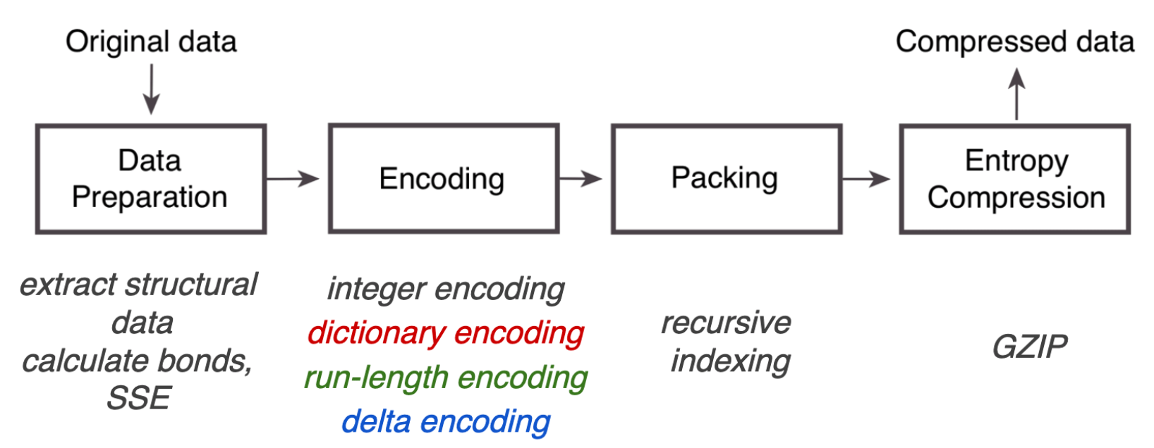
Overview of the MMTF compression pipeline. Source: UCSD Presentation

We can see that after some data preparation, the main steps in the MMTF pipeline are various ways of encoding to reduce the file size:

• integer encoding
• dictionary encoding
• run-length encoding
• delta encoding

After these encodings, the file size is compressed further by packing into the MessagePack format. Its slogan reads like It’s like JSON, but fast and small, indicating its flexiblity in storing data e.g. as key-value pars, but in a binarized format.

MMTF is great for fast transmission of data and rethought quite a lot of things in clever ways. However, it deviated quite a bit from the mmCIF standard and therefore never really caught on in the community. This has now been confirmed, with MMTF being deprecated from July 2024 onward.

BinaryCIF format

There was a need for a binarized efficient format for protein structure information transfer that was more aligned with the PDBx/mmCIF file format specification. Enter Binary CIF, a newer format that is easier to interconvert with the now standard PDBx/mmCIF. The Binary CIF specification is actually quite readable, so I recommend checking it out.

BinaryCIF was heavily inspired by MMTF, with many people working on both formats. This is visible in the usage of MessagePack and the different encodings employed.

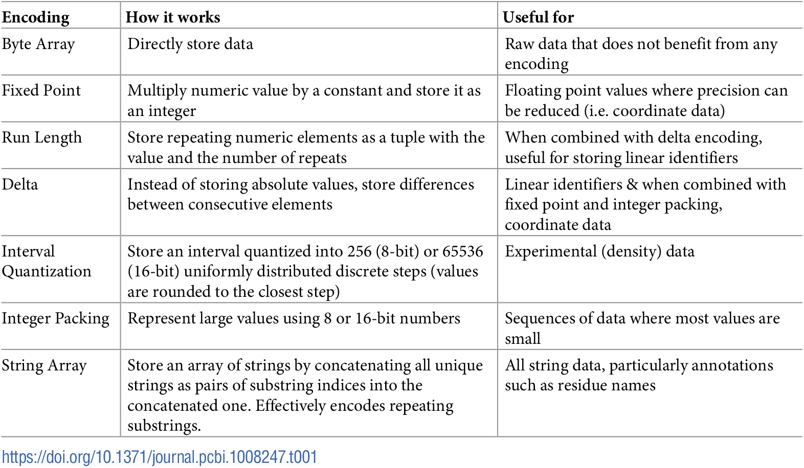
Encodings employed for BinaryCIF. Source: BinaryCIF paper

There are a few additional ones that you can read up on in the specification on GitHub, but mostly the same encodings were used as in MMTF

Input Data for Machine Learning Algorithms

We’ve discussed how protein structures are stored in databases; with that done, let us talk about how they are represented in machine learning algorithms.

Amino acid encodings

Encoding the sequence information into a numerical format should not be too hard; our vocabulary size is only 20 and we do not have to deal with symmetries as we will see later with geometric information like coordinates.

However, if you actually look into different code bases, you will soon find a decade-old problem revived again:

The old ordeal of standardisation. Source: xkcd.com

Depending on which codebase you use, the ordering of amino acids used to encode them into numerical format might be different, introducing the possibility of silent but horrible bugs later down the line. Some alphabets even have a different vocabulary size since they deal with post-translational modifications, non-canonical amino acids or other phenomena you encounter in the wild west of structural biology.

For many applications, people use a de-facto standard by adapting the encoding defined by AlphaFold2. If we look at the OpenFold codebase, we can see that their ordering includes the 20 canonical amino acids together with an unknown residue token represented by X:

# This is the standard residue order when coding AA type as a number.
# Reproduce it by taking 3-letter AA codes and sorting them alphabetically.
restypes = [
    "A",
    "R",
    "N",
    "D",
    "C",
    "Q",
    "E",
    "G",
    "H",
    "I",
    "L",
    "K",
    "M",
    "F",
    "P",
    "S",
    "T",
    "W",
    "Y",
    "V",
]
restype_order = {restype: i for i, restype in enumerate(restypes)}
restype_num = len(restypes)  # := 20.
unk_restype_index = restype_num  # Catch-all index for unknown restypes.

restypes_with_x = restypes + ["X"]
restype_order_with_x = {restype: i for i, restype in enumerate(restypes_with_x)}

OpenFold amino acid encoding.

However, some other models/frameworks use an amino acid encoding that is created by sorting the 1-letter codes instead of the 3-letter codes alphabetically. If in doubt, check which encoding your data uses to avoid confusion.

Coordinates: Atom14 vs Atom37

When looking at either the original AlphaFold codebase or the open-source reproduction in PyTorch called OpenFold, many people trip over how the coordinates from the file formats discussed earlier are represented inside the neural network. This confusion is enhanced by there being two different network-internal representations which are converted into each other depending on the use case scenario.

The documentation on these two representations is sparse, with one being available on a HuggingFace docstring:

Generally we employ two different representations for all atom coordinates, one is atom37 where each heavy atom corresponds to a given position in a 37 dimensional array, This mapping is non amino acid specific, but each slot corresponds to an atom of a given name, for example slot 12 always corresponds to ‘C delta 1’, positions that are not present for a given amino acid are zeroed out and denoted by a mask. The other representation we employ is called atom14, this is a more dense way of representing atoms with 14 slots. Here a given slot will correspond to a different kind of atom depending on amino acid type, for example slot 5 corresponds to ‘N delta 2’ for Aspargine, but to ‘C delta 1’ for Isoleucine. 14 is chosen because it is the maximum number of heavy atoms for any standard amino acid. The order of slots can be found in ‘residue_constants.residue_atoms’. Internally the model uses the atom14 representation because it is computationally more efficient. The internal atom14 representation is turned into the atom37 at the output of the network to facilitate easier conversion to existing protein datastructures.

What does this mean in practice? Let’s look at the code. When looking at residue_constants.residue_atoms, we get the following description for the atom14 representation:

# file: "residue_constants.py"
# A list of atoms (excluding hydrogen) for each AA type. PDB naming convention.
residue_atoms = {
    "ALA": ["C", "CA", "CB", "N", "O"],
    "ARG": ["C", "CA", "CB", "CG", "CD", "CZ", "N", "NE", "O", "NH1", "NH2"],
    "ASP": ["C", "CA", "CB", "CG", "N", "O", "OD1", "OD2"],
    "ASN": ["C", "CA", "CB", "CG", "N", "ND2", "O", "OD1"],
    "CYS": ["C", "CA", "CB", "N", "O", "SG"],
    "GLU": ["C", "CA", "CB", "CG", "CD", "N", "O", "OE1", "OE2"],
    "GLN": ["C", "CA", "CB", "CG", "CD", "N", "NE2", "O", "OE1"],
    "GLY": ["C", "CA", "N", "O"],
    "HIS": ["C", "CA", "CB", "CG", "CD2", "CE1", "N", "ND1", "NE2", "O"],
    "ILE": ["C", "CA", "CB", "CG1", "CG2", "CD1", "N", "O"],
    "LEU": ["C", "CA", "CB", "CG", "CD1", "CD2", "N", "O"],
    "LYS": ["C", "CA", "CB", "CG", "CD", "CE", "N", "NZ", "O"],
    "MET": ["C", "CA", "CB", "CG", "CE", "N", "O", "SD"],
    "PHE": ["C", "CA", "CB", "CG", "CD1", "CD2", "CE1", "CE2", "CZ", "N", "O"],
    "PRO": ["C", "CA", "CB", "CG", "CD", "N", "O"],
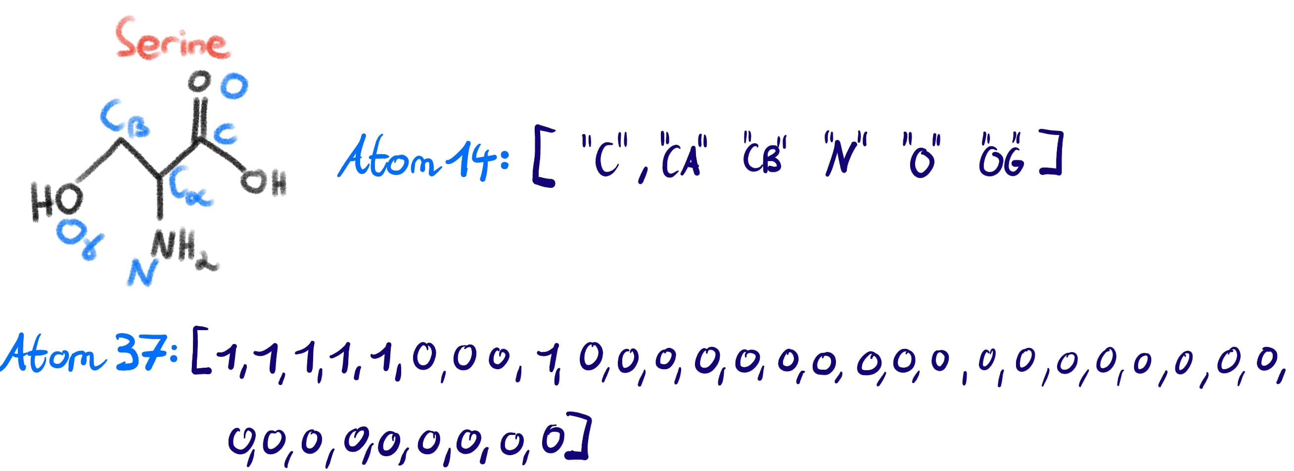
    "SER": ["C", "CA", "CB", "N", "O", "OG"],
    "THR": ["C", "CA", "CB", "CG2", "N", "O", "OG1"],
    "TRP": ["C", "CA", "CB", "CG", "CD1", "CD2", "CE2", "CE3", "CZ2", "CZ3", "CH2", "N", "NE1", "O"],
    "TYR": ["C", "CA", "CB", "CG", "CD1", "CD2", "CE1", "CE2", "CZ", "N", "O", "OH"],
    "VAL": ["C", "CA", "CB", "CG1", "CG2", "N", "O"]}

atom14 ordering.

We see that depending on whch amino acid we have present, a certain position in a residue array can represent a different atom (for example, position 3 is CG2 for Threonine, CG1 for Valine and N for Serine). This makes storing this information very efficient, but can be cumbersome if we need to retrieve the coordinates of a certain atom like N from our data structure.

On the other hand, the atom37 representation has a fixed atom data size for every residue. This ordering can be found in residue_constants.atom_types:

# file: "residue_constants.py"
# This mapping is used when we need to store atom data in a format that requires
# fixed atom data size for every residue (e.g. a numpy array).
atom_types = [
    "N",
    "CA",
    "C",
    "CB",
    "O",
    "CG",
    "CG1",
    "CG2",
    "OG",
    "OG1",
    "SG",
    "CD",
    "CD1",
    "CD2",
    "ND1",
    "ND2",
    "OD1",
    "OD2",
    "SD",
    "CE",
    "CE1",
    "CE2",
    "CE3",
    "NE",
    "NE1",
    "NE2",
    "OE1",
    "OE2",
    "CH2",
    "NH1",
    "NH2",
    "OH",
    "CZ",
    "CZ2",
    "CZ3",
    "NZ",
    "OXT",
]
atom_order = {atom_type: i for i, atom_type in enumerate(atom_types)}
atom_type_num = len(atom_types)  # := 37.

atom37 ordering.

Here we can see that the ordering is always the same no matter which residue is represented; however, most of the fields will always be empty since the longest amino acid (tryptophane) has only 14 atoms. We therefore exchange efficiency for standardisation, which explains why internally AF2 often uses atom14, but when it interfaces to other programs at I/O it often uses atom37.

If we think about our example of Ser again, we can see how the machine representations map to the actual amino acid (again with the caveat that hydrogens are ommited and the carboxyl oxygen is not counted since in a peptide backbone it will have let as water).

Category	Atom14	Atom37
Memory Requirements	Efficient	Wasteful
Data Layout	Varying Shape	Fixed Shape
Sequence Dependence	Yes	No

Boundary Conditions: OXT

I have been talking before about the oxygen atom of the carboxy group that is lost when two amino acids combine to form a peptide bond. Well, that is true for all amino acids except the last one at the C-terminus since there the carboxy group will still be free and has two oxygen atoms. At physiological pH the carboxy group will be deprotonated so both oxygen atoms are chemically equivalent with equal bond lengths (as opposed to the single and double bond image we always draw on paper), but our file formats still require us to name one of the oxygens at the terminus as a “normal” oxygen, i.e. O and the other one OXT. You will therefore often see the last atom in a protein structure being OXT, such as in this Biopandas tutorial. When I say “often”, I mean “not always”; the termini of protein are known to often be too flexible to crystallise, therefore the structure in our PDB files will often end prior to the C-terminus and not contain an OXT. This is not super problematic since given the planarity of the delocalised carboxy electron system, one can place the OXT easily given the carbon and the other oxygen atom. Predicted structures such as the ones from AlphaFold2 on the other hand will always contain the OXT atom since they do not have to battle experimental resolution problems.

Example: Lysozyme atom numbering

Let us now visualise the concepts we looked at so far (atom names and atom representations) with a concrete example, again based on the lysozyme structure with the PDB code 168l. Install PyMol (either the commercial or the open-source version) and open the program.

If you have not used PyMol before, you can either skip this section or look at this lesson from my Structural Bioinformatics course that goes over this in detail.

Then, execute the following commands via the integrated terminal:

fetch 168lA # get first chain of lysozyme assembly
select selection, resi 11-15 # select a subset of residues for simplicity
hide everything # hide the whole structure for clarity
show sticks, selection # show stick representation for the selected subset; carbon is green, oxygen is red, nitrogen is blue
color yellow, (name CG) # color all CG atoms yellow
color orange,  (name NH1) # color the single NH1 atom orange

After doing this, you should see something like this:

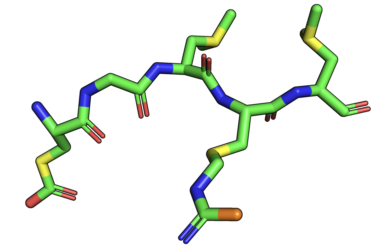
We can compare this to a schematic sketch of this protein segment, similar to what we did before with serine:

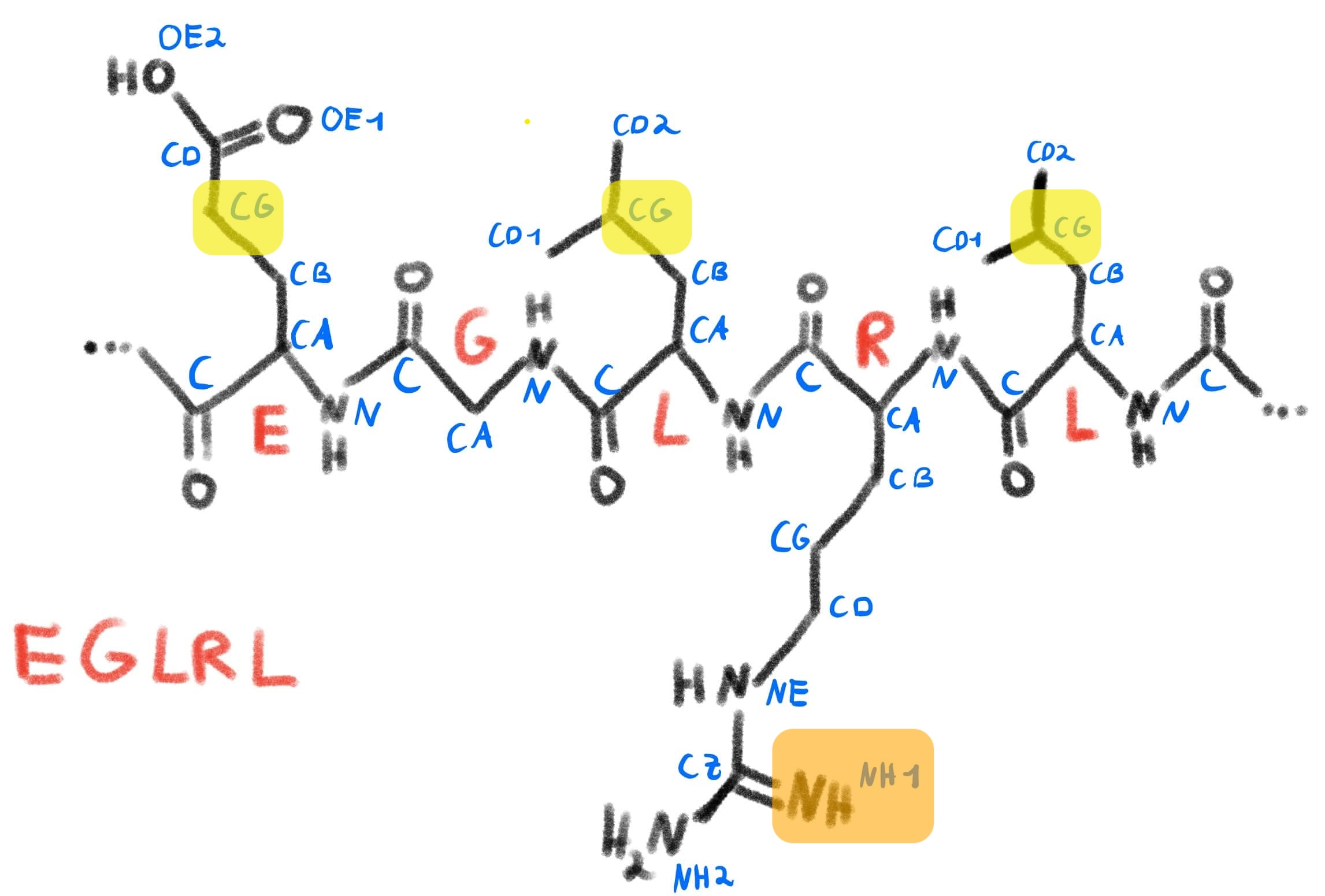
Schematic representation of the selection from our protein, with the coloring imitating our color scheme in PyMol.

We can see that PyMol knows about the atom naming convention we discussed and can select and color residues accordingly. It does this by parsing the information it gets from the PDB file and storing this inside the structure object it displays.

We can do the same thing programmatically by using a library such as Biotite.

import biotite.structure as struc
import biotite.structure.io.mmtf as mmtf
import biotite.database.rcsb as rcsb

mmtf_file = mmtf.MMTFFile.read(rcsb.fetch("168l", "mmtf"))
structure = mmtf.get_structure(mmtf_file, model=1)

chain_A = structure[
    (structure.chain_id == "A") & (structure.hetero == False)
]
print(chain_A.res_id) # array([  1,   1,   1, ..., 164, 164, 164])
selection = chain_A[(chain_A.res_id > 10) & (chain_A.res_id <= 15)]
print(selection.res_id) # [ 11 11 ... 15 15 ]
print(selection.array_length()) # 40

We see that our selection contains 40 atoms. We can check if that corresponds to the amino acids we wanted to select by checking how many non-hydrogen atoms each of these amino acids have and by subtracting on average 1 oxygen atom per amino acid for the formation of the peptide bond.

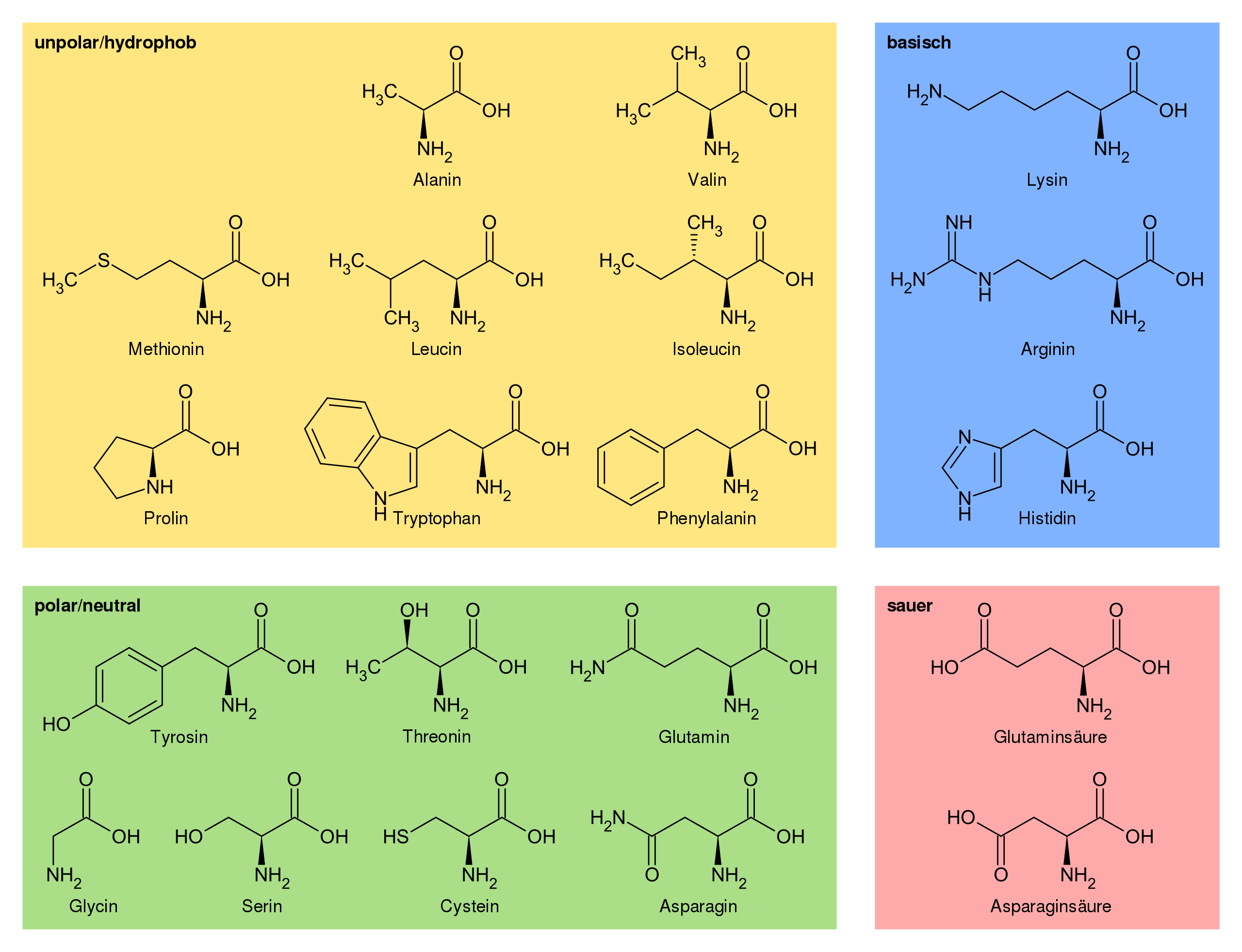
Proteinogenic amino acids and some of their properties. Source: Wikipedia $$\begin{align} E + G + 2L + R - 5 &= 10 + 5 + 2*9 + 12 - 5 &= 40 \end{align}$$

Reference Systems: Local reference frames vs reference-free methods

We now have covered how we go from the database formats for protein structures (PDBx/mmCIF, MMTF and BinaryCIF) to the formats commonly used as inputs for machine learning models (atom14, atom37). The question now is: what do the machine learning models do with this input information?

Given that we deal with geometric quantities such as coordinates of protein structures, considerations like invariance and equivariance come into play. There is a whole field called Geometric Deep Learning that deals with with these considerations. For the usage of machine learning models for protein structure, it is important to understand the distinction between reference-free and reference-based methods.

To learn more about geometric deep learning, you can either check out the protobook by Bronstein et al., the Hitchhiker’s guide to geometric GNNs or this lecture I gave on the topic.

If we predict some molecular property (such as binding affinity, solubility or immunogenicity) it is quite obvious to a human that rotations or translations of the protein should not change the prediction of these quantities. A neural network, however, just sees different numbers when a protein is translated and therefore needs to learn that these different inputs correspond to the same protein. This can be done via data augmentation, but this can become data-inefficient. Therefore, people looked for ways to build this inductive bias of invariance or equivariance to SE(3) group actions (i.e. rotations and translations) into the model.

Local reference-based methods

On one hand, some models leverage reference-based methods, largely following the example of the original AlphaFold2 model. Here, a local reference frame for each residue is defined based on the backbone geometry, with the translational component being equal to the CA position and the rotational component originating from a Gram-Schmidt orthogonalisation with respect to the CA-C and the CA-N bond vector.

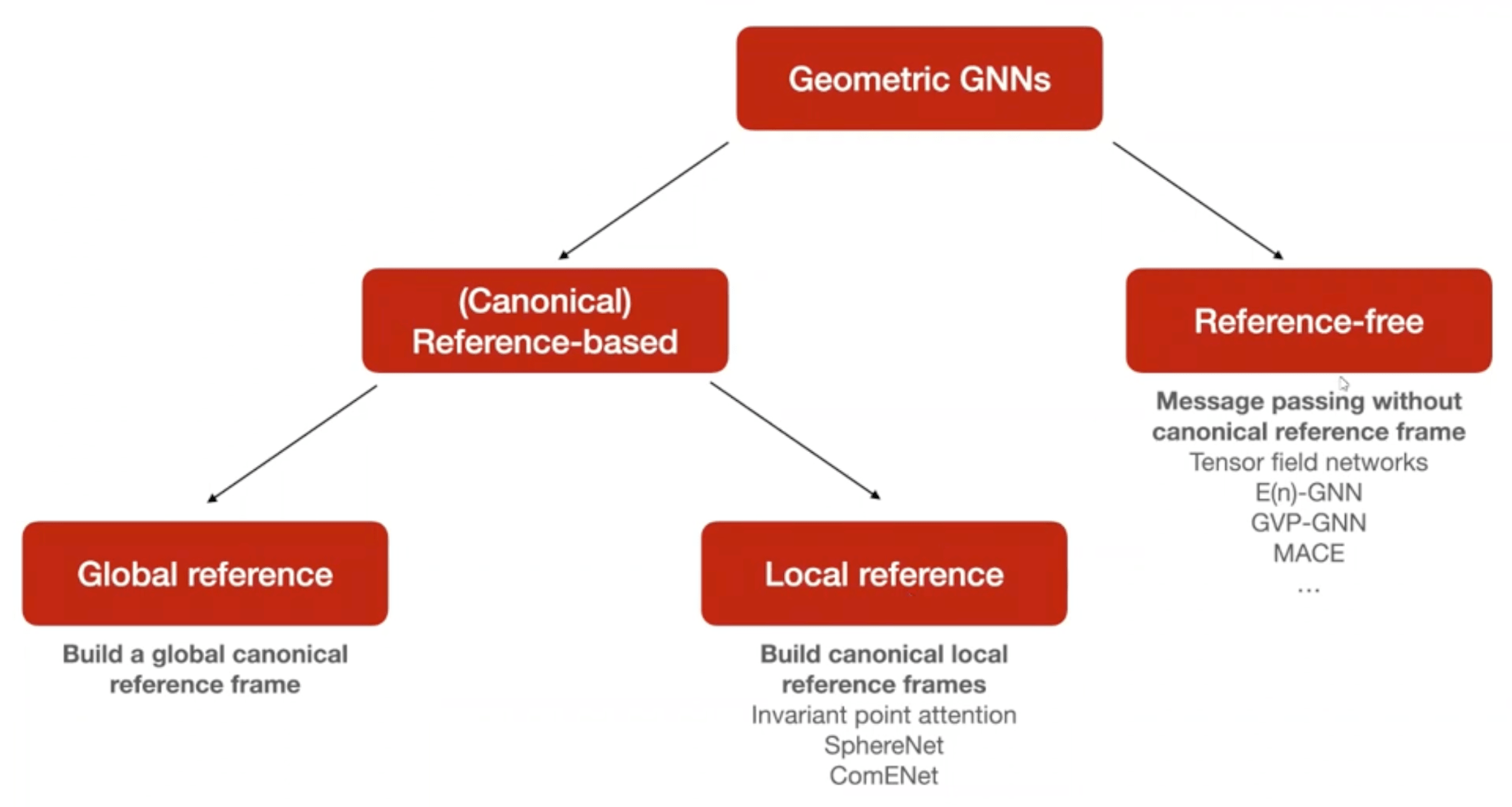
Here a paragraph from the Hitchhiker’s Guide to Geometric GNNs for 3D Atomic Systems that summarizes the current state in this field of research:

Canonical frame-based invariant GNNs. Canonical frame-based GNNs [Liu et al., 2022, Wang et al., 2022a] use a local or global frame of reference to scalarise geometric quantities into invariant features which are used for message passing, offering an alternative technique when canonical reference frames can be defined. Most notably, the Invariant Point Attention layer (IPA) from AlphaFold2 [Jumper et al., 2021] defines canonical local reference frames at each residue in the protein backbone centred at the alpha Carbon atom and using the Nitrogen and adjacent Carbon atoms. Other invariant GNNs for protein structure modelling also process similar local reference frames [Ingraham et al., 2019, Wang et al., 2023b]. IPA is an invariant message passing layer operating on an all-to-all graph of protein residues. In each IPA layer, each node creates a geometric feature (position) in its local reference frame via a learnable linear transformation of its invariant features. To aggregate features from neighbours, neighbouring nodes’ positions are first rotated into a global reference frame where they can be composed with their invariant features (via an invariant attention mechanism), followed by rotating the aggregated features back into local reference frames at each node and projecting back to update the invariant features.

These canonical local reference frames $T = (r, x) \in \text{SE(3)}$ can be used to deal with quantities in a SE(3)-invariant way. Importantly, the orientational nature of the frame allows us to be SE(3)-invariant but not E(3)-invariant, i.e. reflections are still accounted for. This is important for biological applications since chirality plays a huge role in biomolecular interactions.

Why SE(3) instead of E(3) equivariance can be important

As an example of why this is important, we can look at the task of protein structure prediction that AlphaFold2 tackled.

To learn more about AlphaFold2 and the problem of protein structure prediction, you can either check out the 3-part lecture series about AF2 by Nazim Bouatta or this lecture I gave on the topic.

Here, one important metric for measuring prediction accuracy is the GDT score. To get good at maximising this score, a natural way to think about it is to take your predicted coordinates, compare them to the ground-truth coordinates and compute something like an RMSD loss. However, this does not take rototranslations into account of course. We can remedy that by calculating a dRMSD loss, i.e. a RMSD loss on all pairwise distances in the structure. By using these internal coordinates, we are invariant to rototranslations.

However, we are also invariant to reflections! When training AlphaFold2, the team at DeepMind tested what would happen if they used this dRMSD loss for training a model.

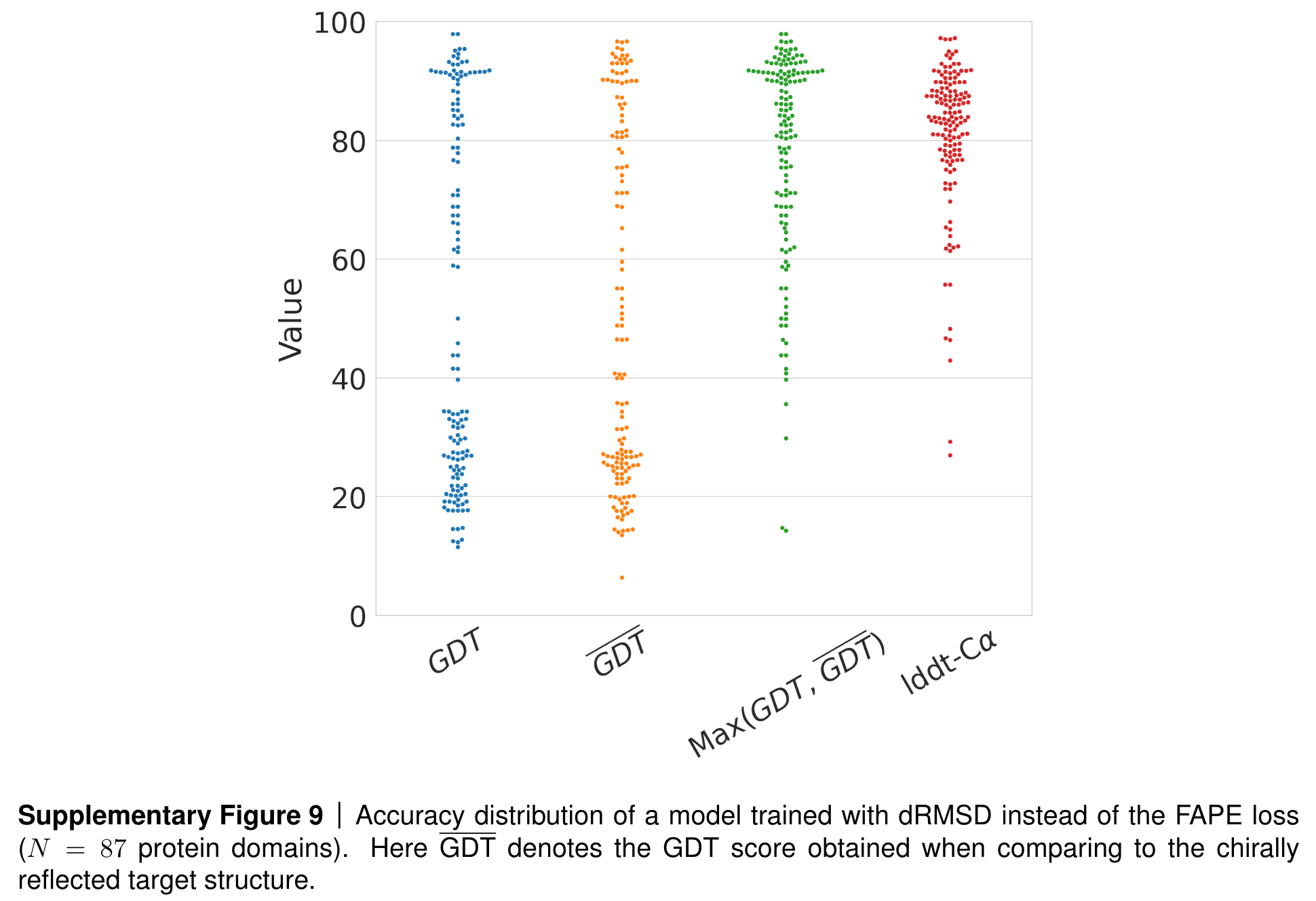
Results if AF2 is trained with dRSMD instead of FAPE as loss. Source: AF2 SI, page 36, section 1.9.3.

You can see that while the local structure of predicted proteins (as measured by the lddt-CA score) seem very good, the global structure (as measured by the GDT score) seems to follow a bimodal distribution, with half the predictions performing well and the other half faring badly. Could this be due to the reflection invariance of the dRMSD loss? When calculating the GDT score with respect to the mirror image structure, the team observed a reversal of the distribution! Finally, when looking at the maximum of these two scores (one calculated with respect to the ground truth structure and one with respect to its mirror image), the model shows strong performance, indicating that the issue was indeed the reflection-invariant dRSMD loss.

Here frames come to our rescue and allow the definition of the so-called FAPE loss (frame-aligned point error, minimal implementation here). With their help, we can compute distance-like quantities, but in a reflection-aware way. How do we do that? We can take a predicted position $x_j$ and compute its position relative to the predicted frame of a different residue $T_i$. With this, we effectively get a displacement vector which is however reflection-aware due to the rotational component of the frame transformation.

We can do the same thing for the ground-truth positions and frames that can be computed for the same combination of residues and score the difference as a RMSD-like quantity. This is what the FAPE loss amounts to.

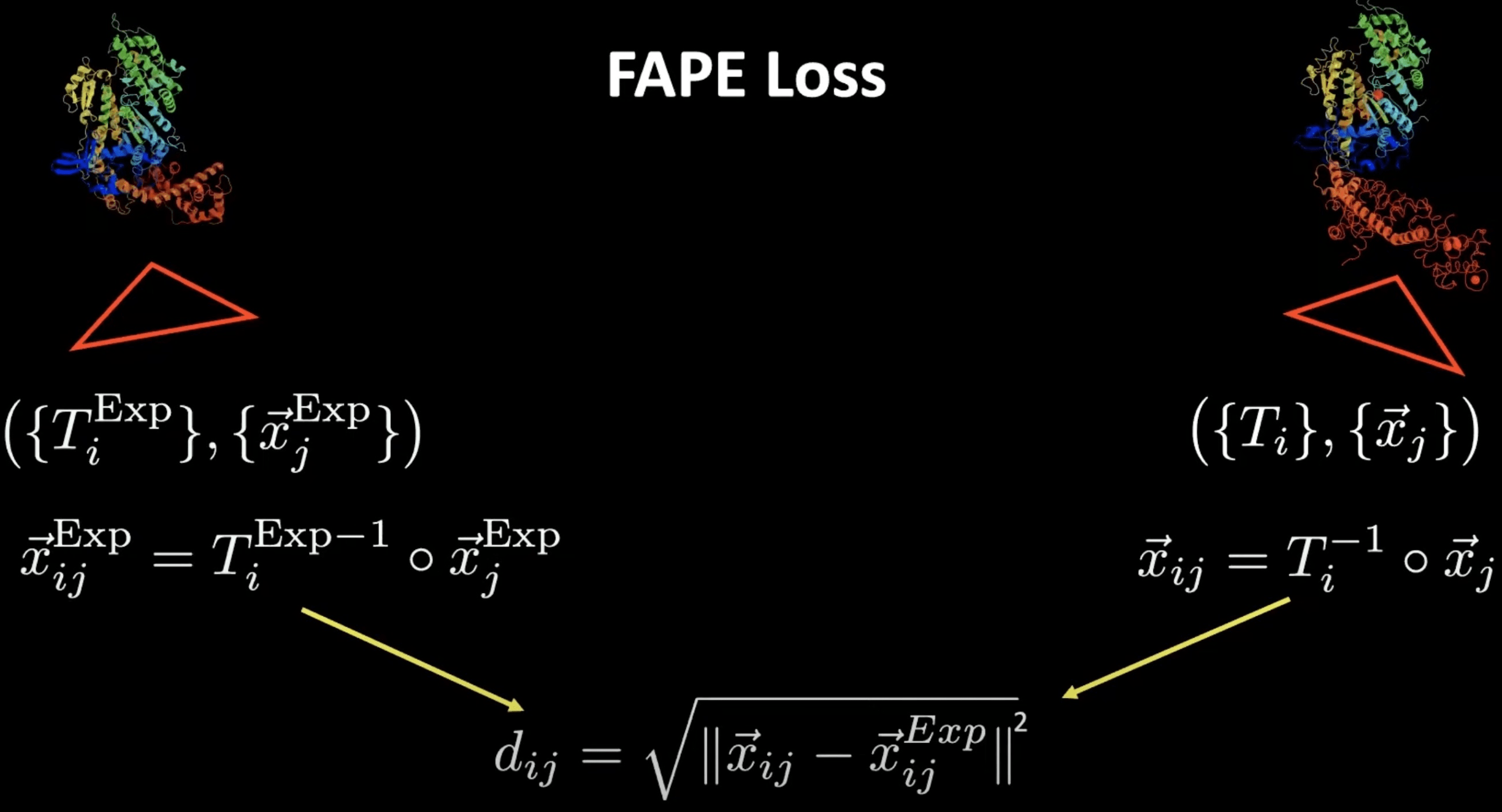
FAPE loss visualisation for a single pair of residues. Source: YouTube talk at HMS.

An equivalent way of visualising this involves not looking at a single pair of residues, but considering it in the context of the whole structure. Here, we align the predicted and the target structure based on frame $T_i$ and then calculate the L2 norm of all the other residues with respect to this specific alignment. We can then repeat this for all residues in the sequence to calculate the overall FAPE loss.

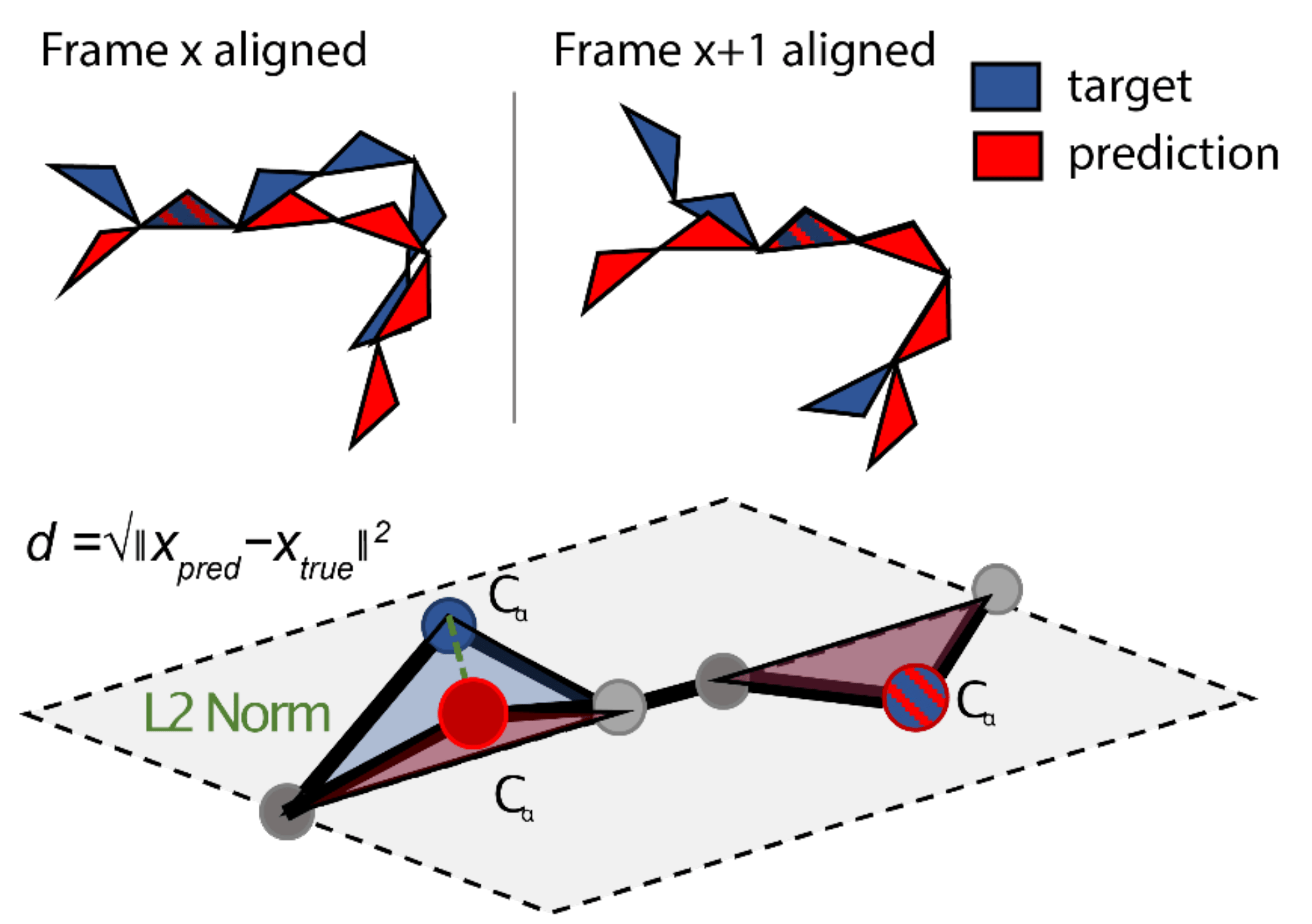
FAPE loss in the context of the whole structure. Source: AF2Seq paper.

Note that there are different versions of the FAPE loss used in different parts of the model; while the final FAPE loss computes these L2 norms for all atoms, the intermediate FAPE loss only considers the CA positions.

This type of frame definition is by no means the only way you can construct frames; RGN2, another model for protein structure prediction instead uses Frenet–Serret frames to model the protein backbone.

Ambivalent mappings from frames to coordinates

At the end of AlphaFold2, the algorithm has to again map the frame-based representation into 3D coordinates. This should not be a problem since we have our backbone frames that allows to reconstruct the backbone positions, and we predict the torsion angles of the rigid groups in the side chains so that we can place all atoms correctly according to the following table.

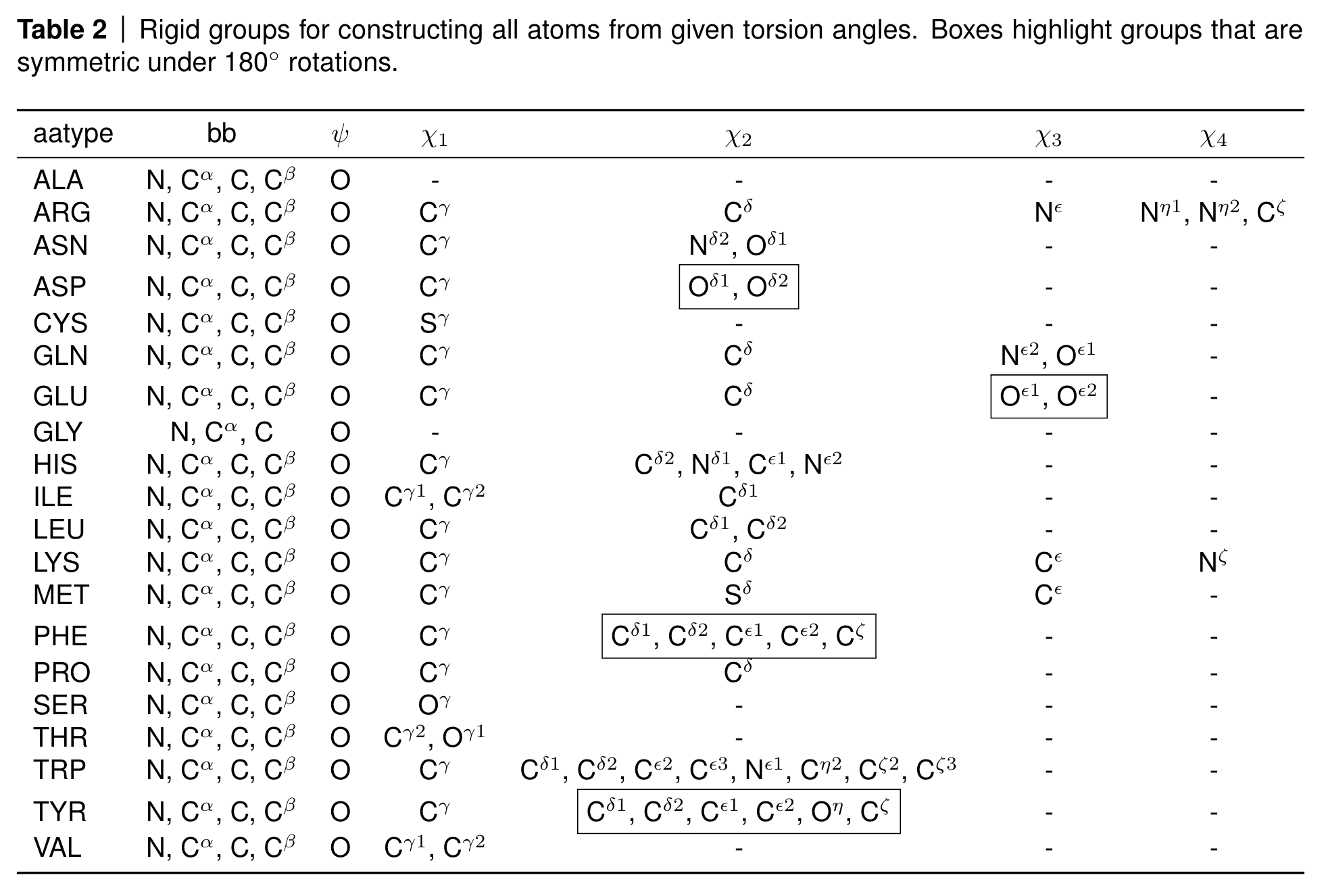
Rigid groups for constructing all atoms from given torsion angles. Source: AF2 SI, Table 2

However, you can see a few boxed atoms in the table. These atoms are symmetric under 180 degree rotations, such as five of the six atoms in the phenyl ring of phenylalanine (PHE) and tyrosine (TYR) or the terminal carboxyl oxygens in asparagine (ASP) and glutamate (GLU).

Some of these atoms are on the rotation axis such as the terminal carbon atom in the phenyl rings and are therefore invariant to the rotation; some of the other atoms however swap positions due to the 180 degree rotation symmetry and their atom names are therefore ambiguous.

AlphaFold deals with this by renaming the atoms in a globally consistent way via lDDT loss computations (see algorithm 26 in the SI and this part of the OpenFold codebase).

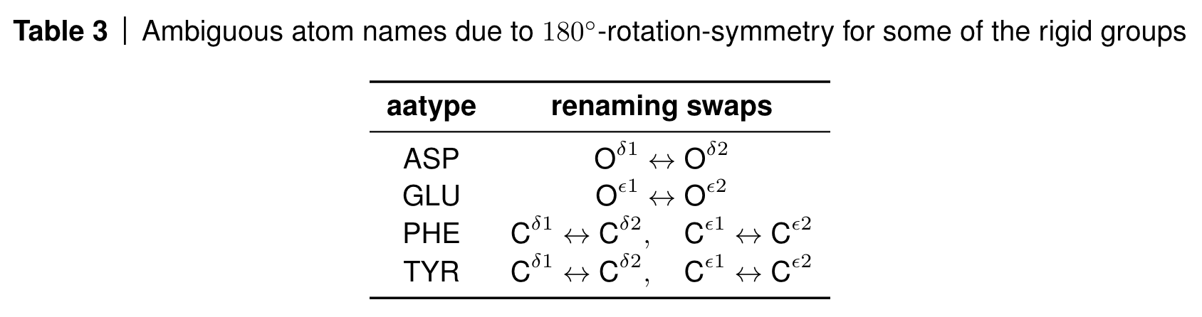
Renaming convention for ambivalent atom placements. Source: AF2 SI, Table 3

Another problem that comes from this ambiguity is that the network can in theory predict to valid values for the torsion angle of these rigid groups, $\chi$ as well as $\chi + \pi$. AlphaFold therefore allows the network to predict both angles by giving it both the predicted and the possible alternative angle (in the case of non-symmetric configurations, they are both set to the predicted value). In this way, the network is allowed to learn both valid values.

Reference-free methods: Invariant and Equivariant Update Functions

We do not necessarily need to represent our structures as frames where we define a local reference coordinate system, but can also directly operate on our coordinates as long as we update our representation at every layer in a way that properly leverages these symmetries (e.g. by SE(3) invariance or equivariance).

Examples that leverage this approach include GVP-GNN which defines equivariant update functions as well as SchNet and DimeNet that leverage invariant update functions (message passing functions in GNN-speak).

To learn more about how these different approaches can be classified, I recommend both this paper as well as the Hitchhiker’s guide to geometric GNNs.

Leaving the GNN camp for a bit, Ophiuchus showed that one can use hierarchical autoencoders to operate over protein structures which are represented by CA atoms and geometric features attached to them that describe the other atomic positions. They employ SE(3)-equivariant convolutions to operate on this representation and demonstrate its usage for compression and structure generation.

Screw these symmetries: data augmentation and other strategies

Frame-based representations have been successfull in AlphaFold and have since been used in many other models, both supervised and generative, for example RFDiffusion and Chroma. However, defining things like diffusion processes over these frames becomes quite a bit harder, and if you additionally deal with sidechains and other details, frames might be too cumbersome for your use case.

Other models therefore do not use frames, but some kind of internal coordinates that can be used without explicitly considering these symmetry constraints. Some examples of this include RGN and FoldingDiff that leverage torsion angles or ProteinSGM that leverages a mixture of torsion angles and backbone distances.

Another strategy that does not involve dealing with symmetries is - well, not dealing with symmetries. Protpardelle is a protein diffusion model that operates on pure coordinate representations via a vision transformer and does some rotational and translational data augmentation to account for these symmetries. Finally, in the small molecule world, the Molecular Conformer Fields paper showed that empirically, not enforcing these symmetry constraints explicitly can still lead to SOTA performance, sparking quite a discussion on Twitter.

Batching: Padded versus sparse

We’ve now covered the whole pipeline, starting from database formats over input formats to network-internal representations to properly handle symmetries. A final consideration comes into play when we think about batching, a commonly used technique in machine learning where you do not pass your samples one by one into the network, but combine them into a bigger tensor to achieve better hardware utilisation and therefore training performance.

There are many subtleties to choosing your batch size since generally we perform a gradient update step after each of these batches; therefore, the batch size not only influences training performance but also accuracy by changing the dynamics of our gradient descent procedure. I won’t go into detail here on that, but recommend Andrej Karpathy’s blog on general recipes for training neural networks.

The batching pain with variable-length input

This batching of tensors is trivial in many computer vision use cases since often all your images are of the same size; you can therefore just stack them along a new dimension and ready is your batch.

For protein structures, it is a bit more complicated due to variable length. One strategy to deal with this involves padding and trunction. Here, we choose some maximum length for our batch and pad structures that are shorter than this via padding tokens (for coordinates this can be 0 or a small value that is unlikely to occur exactly like this in the data) and truncate structures that are longer than this (either randomly or via some biologically defined domain boundaries). This solves our issue, but introduces new ones: often, we do not want to truncate data since we may lose important information. If we now always choose the longest structure in a batch as the maximum length, we may end up with very inefficient training if there are very short sequences in the batch and padding tokens begin to represent a significant part of our batch.

Efficient padding via length batching

To circumvent this, people took inspiration from NLP. In the transformer paper, for example, it is stated that to circumvent the inefficient padding issue, sentence pairs were batched together by approximate sequence length, resulting in more optimal padding. This has been replicated for example in generative models for protein structure. This change might influence training dynamics since now the model sees similarly-sized inputs inside every batch, but empirically still seems to work fine.

Sparse batching

In the previous section we talked about the usage of GNNs (graph neural networks) for protein structures. A popular library in the field of GNNs is PyG (PyTorch Geometric) that can be used for all kinds of graph-structure data.

In contrast to the padding-and-truncation approach I mentioned before, they opt for a sparse batching procedure they term advanced mini-batching.

Here, we treat the our graph data points in a batch as one single datapoint and use pointers to tell us about the boundaries between these. In practice, we concatenate all our node features along an existing dimension instead of stacking them along a new dimension, making padding and truncation obsolete.

Advanced mini-batching in Pytorch Geometric. Source: PyG Docs

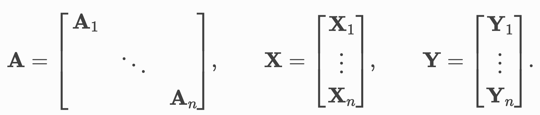
We do something similar for the adjacency matrix which indicates the connectivity in the graphs. Stacking these in a block-diagonal fashion allows us to reuse existing algorithms for GNNs such as message-passing without having to change implementations. In addition, since the majority of elements in this matrix will be zero, we can use sparse representations that allow us to deal with this in a memory-efficient way.

If you inspect protein structures represented in this PyG format (such as in the ProteinWorkshop project we recently published), you can see that a graph will look like this:

DataBatch(
  coords=[7241, 37, 3],
  residues=[32], 
  residue_id=[7241], 
  chains=[7241], 
  seq_pos=[7241, 1], 
  batch=[7241], 
  ptr=[33])

In contrast, this same batch in the “dense” format that uses padding would look like this:

DataBatch(
  coords=[32, 385, 37, 3],
  residues=[32],
  residue_id=[32, 385],
  chains=[32, 385],
  seq_pos=[32, 385, 1])

We can notice several differences:

• the dense format represents the batch as an explicit tensor dimension (first dimension of size 32) in all attributes. This dimension is not apparent in the PyG batch except for the attributes that are graph-level attributes and therefore do not change with the size of the graph (residues is an example here, for each graph it is a single list).
• we can see in the dense batch that the longest protein structure in this batch is 385 residues (apparent in for example the residue_id attribute, a numerical encoding of the amino acid type). In the PyG batch, we can see that stacked together all amino acids in the batch sum to 7241. If you compare 7241 to 32*385 = 12320, we can see that padding introduces around 40% of memory overhead compared to the efficiently batched representation.
• the PyG batch stores the batching information not in a separate dimension, but in separate attributes: batch indicates for each node in the batch to which graph in the batch it belongs, and ptr contains pointers to the boundaries between all the graphs in the batch to enable efficient indexing and information retrieval.

Interconversion from dense to PyG format and back is easy to do if all of the graphs are the same size: we can use the PyG DenseDataLoader for that.

In the padded case, there is no such functionality yet, but there might soon be a DensePaddingDataLoader that does exactly that.

AFDB, ESMAtlas & co: how to deal with large databases

The PDB as a database of experimental protein structures keeps growing, currently standing at nearly 218k entries. However, it seems small compared to the AlphaFoldDB (>200m) and ESMAtlas (772m structures), powered by the recent advances in protein structure prediction via methods like AlphaFold2 and ESMFold.

This development changed the game in protein biology. While until recently the gap between available protein sequences and structures widened further and further, we suddenly have a wealth of structural information that was unimaginable a decade ago. This quote from Mohammed AlQuraishi (Columbia University) sums up this paradigm shift well:

Everything we did with protein sequences we can now do with protein structures

While that is a theoretically true and very exciting prospect, there is one big problem: we do not have tools to deal with such amounts of structural data. Here a visual comparison between the size of the PDB and the AFDB:

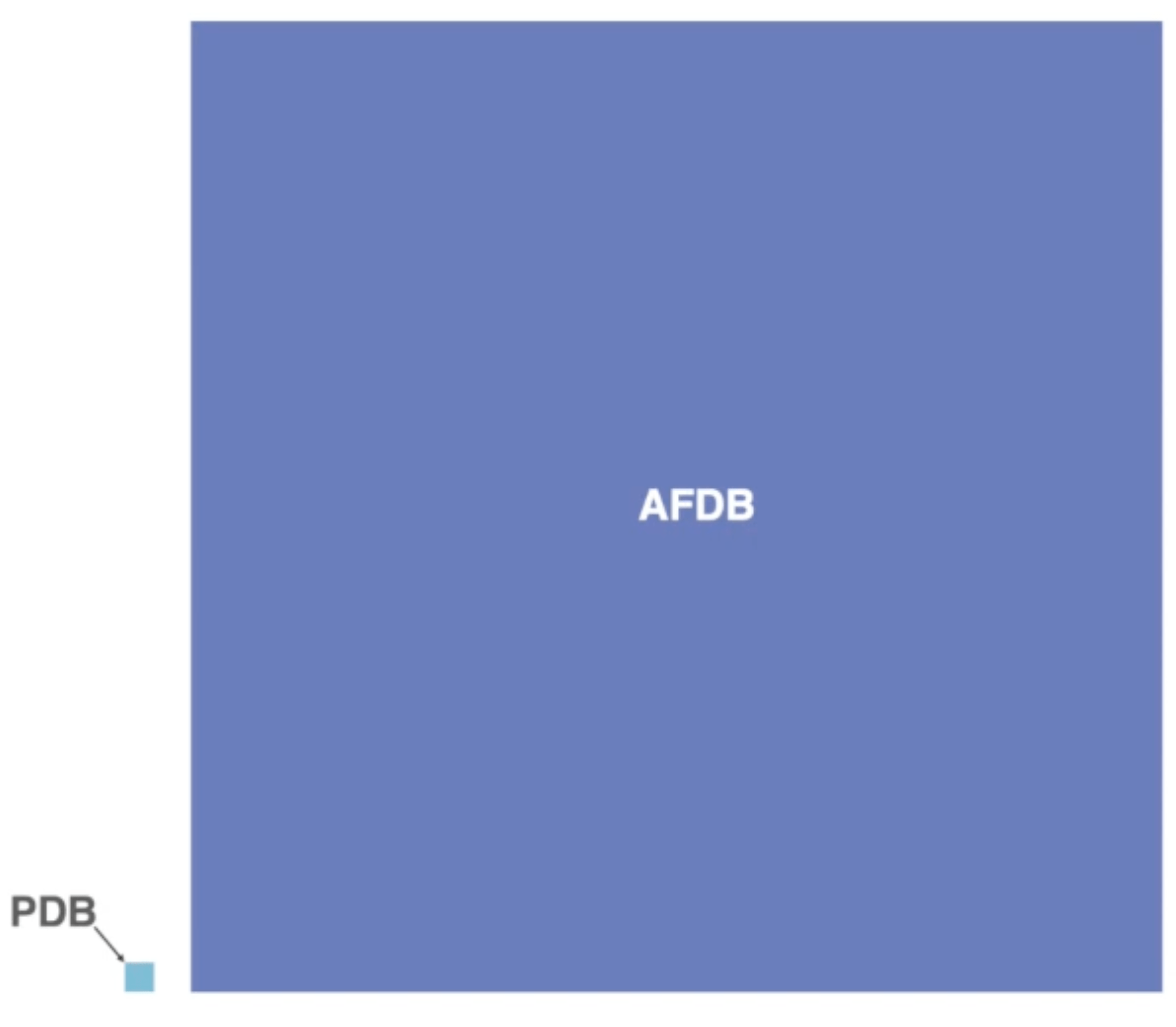
Visual comparison of the size of the PDB vs the AFDB. Source: YouTube

You can see that we deal with a different order of magnitude in data here. This brings up a plethora of issues, starting from pure memory usage (the storage for AFDB is 23 TB) to questions of how we move these enormous amounts of data and also process them.

Many groups have developed tools in the last years to tackle this issue. Especially the Steinegger lab has produced some fantastic tools in that space from which I want to present three here in this blogpost: Foldcomp for structure compression, Foldseek for structure clustering and mmseqs for sequence clustering (also very important in that context for generating both input MSAs and training splits).

Many groups have developed tools in the last years to tackle this issue. Especially the Steinegger lab has produced some fantastic tools in that space. If you want to read more about these tools, I have a separate blogpost describing three of them in detail: Foldcomp for structure compression, Foldseek for structure clustering and mmseqs for sequence clustering (also very important in that context for generating both input MSAs and training splits).

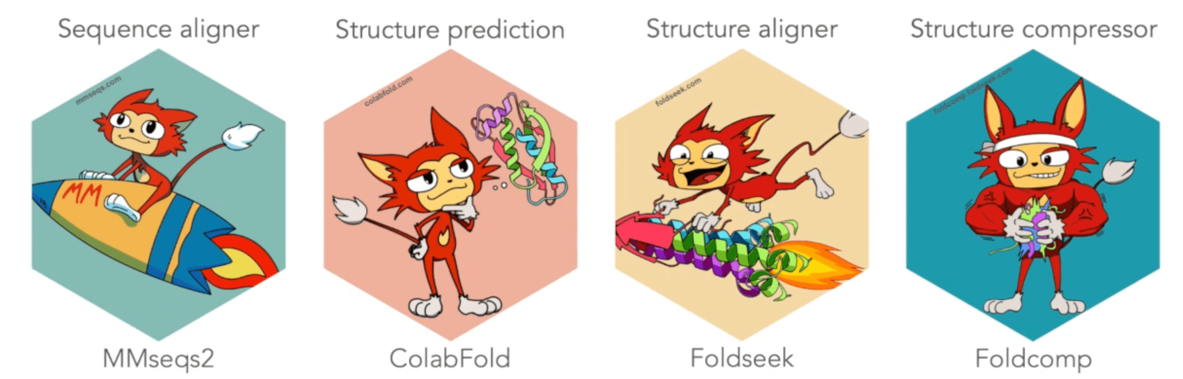
Tools from the Steinegger Lab. Source: YouTube

Summary

In this post we discussed four different levels of information representation:

1. We started with the data formats in which protein structures are stored and transmitted and the evolution they underwent in the last decades.
2. After that we looked at how both sequence and structure information can be converted into a format that can be used by machine learning algorithms, specifically the atom14 and atom37 format.
3. Once inside the network, we discussed how different methods leverage this information differently, either via reference-based or reference-free methods, looking at how we can deal with geometric information while respecting the symmetries inherent to it.
4. Finally, we looked at how different frameworks deal with the variable length of protein structures and how this affects batching behaviour.

I hope that this post can shine some light not only on which representations are used in which circumstances but also why. If you have feedback let me know!