How to accelerate PyTorch on your GPU

A bit of background on GPU acceleration and how to use it with PyTorch
Recently the CUDA MODE lecture series started with some amazing talks about how you can use tools like CUDA or Triton to speed up your PyTorch programs (join the Discord in case you are interested to learn more). Here I want to summarise and review some of the concepts and tools from the lecture and write them together in a coherent blog post.
- 1. Profiling
- 2. Integrating CUDA kernels into PyTorch
- 3. Integrate Triton kernels into PyTorch
- 4.
torch.compile - Credits
1. Profiling
Profiling is the process of measuring the time and resources that a program uses. It is a crucial step in the development of any software, as it allows you to identify bottlenecks and areas for improvement. In the context of GPU programming, profiling is especially important, as the performance of a GPU program can be highly dependent on factors such as memory access patterns, kernel launch configurations, and the specific hardware being used. It is also not trivial to profile GPU code, as the operations are executed asynchronously on the GPU and we cannot simply measure execution time like we would with CPU code. In the following sections are a few tools to get you started on that for PyTorch code (for this you need to have access to a GPU, e.g. via Google Colab or a local machine with a CUDA-enabled GPU).
1.1 torch.cuda.Event
To profile the time a torch opertion takes, you can use torch.cuda.Event. We cannot use the time module for this, because the operations are executed asynchronously on the GPU. Let us write a short function to profile the time a function call takes:
import torch
def time_pytorch_function(func, input):
    start = torch.cuda.Event(enable_timing=True)
    end = torch.cuda.Event(enable_timing=True)
    # Warmup
    for _ in range(5):
        func(input)
    start.record()
    func(input)
    end.record()
    torch.cuda.synchronize()
    return start.elapsed_time(end)
We do a few warmup steps at the start to make sure that things like memory allocation calls, PyTorch’s JIT fuser and other things are not included in the timing. Then we record the start and end of the function call and synchronize the GPU to make sure that the timing is correct. For more details on these things see this blog post.
Let’s try this with a simple toy example:
b = torch.randn(100000, 100000).cuda()

def square_2(a):
    return a * a

def square_3(a):
    return a ** 2

print(time_pytorch_function(torch.square, b))
print(time_pytorch_function(square_2, b))
print(time_pytorch_function(square_3, b))
#output:
# 3.2753279209136963
# 3.272671937942505
# 3.2755520343780518
We can see that the multiplication a * a is slightly faster than the power operation a ** 2. However, we have no idea why this is happening; it is the same operation, so are they using different CUDA kernels? We can use the torch.autograd.profiler to find out.
1.2 torch.autograd.profiler
Fortunately, we do not have to write all profiling tools ourselves PyTorch has a built-in profiler. Let us look again at the same operations:
print("=============")
print("Profiling torch.square")
print("=============")

# Now profile each function using pytorch profiler
with torch.autograd.profiler.profile(use_cuda=True) as prof:
    torch.square(b)

print(prof.key_averages().table(sort_by="cuda_time_total", row_limit=10))

print("=============")
print("Profiling a * a")
print("=============")

with torch.autograd.profiler.profile(use_cuda=True) as prof:
    square_2(b)

print(prof.key_averages().table(sort_by="cuda_time_total", row_limit=10))

print("=============")
print("Profiling a ** 2")
print("=============")

with torch.autograd.profiler.profile(use_cuda=True) as prof:
    square_3(b)

print(prof.key_averages().table(sort_by="cuda_time_total", row_limit=10))
This gives us the following output:
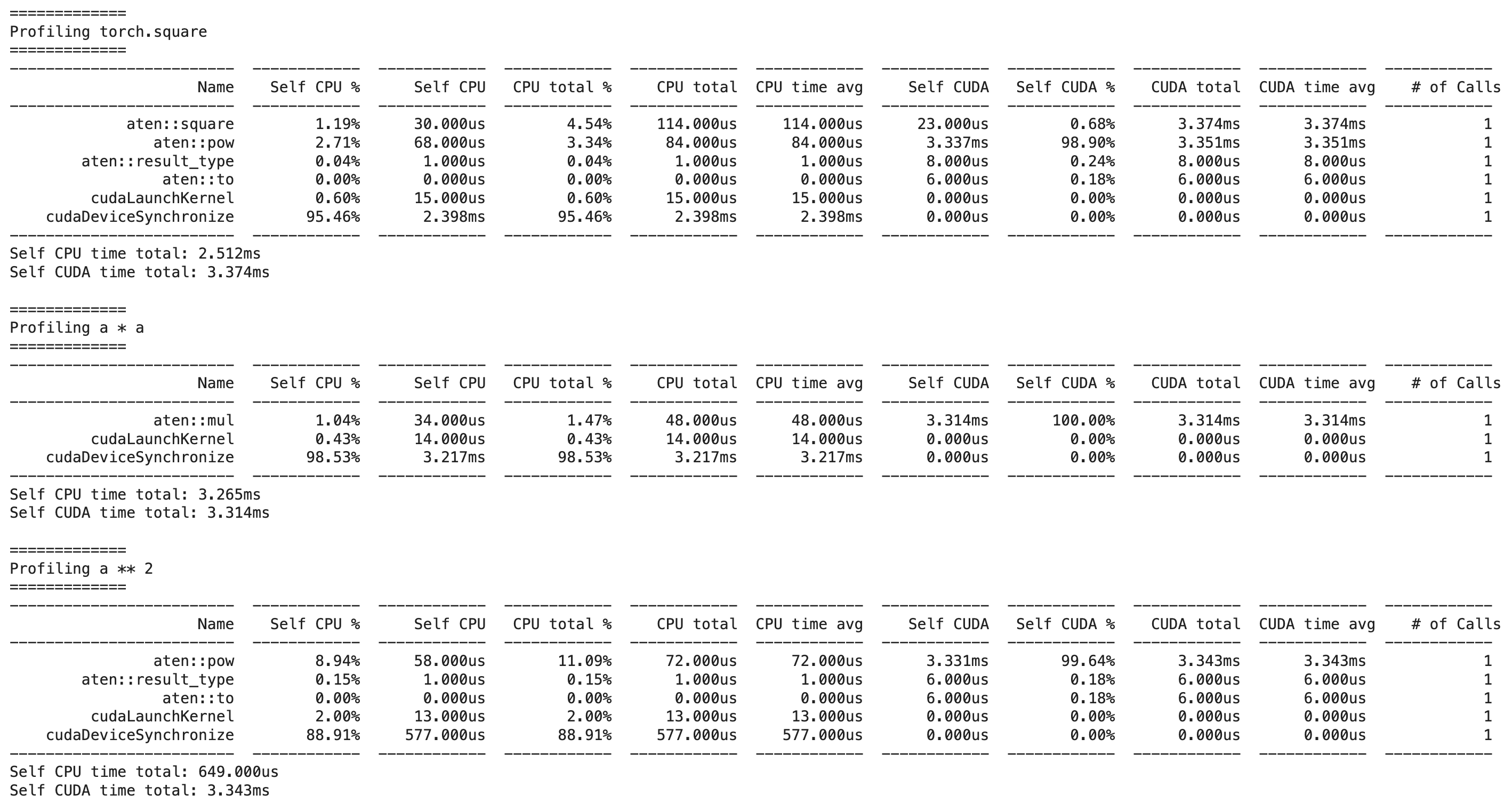
We can see that a * a calls the faster aten::mul operation, while a ** 2 calls the slower aten::pow operation, explaining our previous results.
ATen is a C++ library that is part of the PyTorch C++ API. It is the foundational tensor and math library on which PyTorch is built and exposes the Tensor operations in PyTorch directly in C++. ATen is a very creative name, as it stands for “A tensor library”. You can here more about the differences between the torch API and the ATen API in this podcast episode.
Let us now profile a simple neural network forward pass:
import torch
import torch.nn as nn
import torch.nn.functional as F

data = torch.randn(1, 1, 32, 32).cuda()
with torch.autograd.profiler.profile(use_cuda=True) as prof:
  output = torch.nn.Linear(32, 32).cuda()(data)
print(prof.key_averages().table(sort_by="cuda_time_total", row_limit=10))
Which gives us the following output:
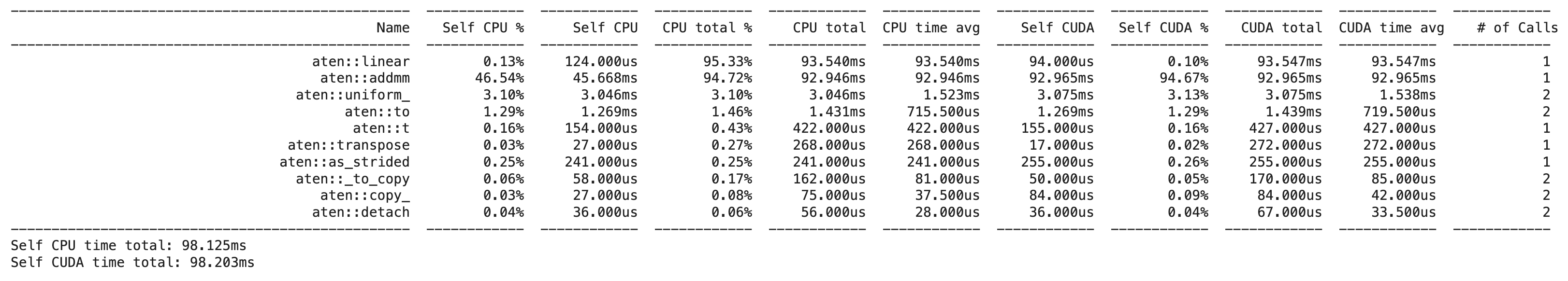
We can see that the aten::linear and the aten::addmm operation are the most time-consuming operations in this forward pass. In another post I dig into how one can find the actual implementation of these functions in the PyTorch codebase to understand what they actually do, but for it is enough to know that aten::linear is the operation that applies a linear transformation to the input data and aten::addmm is the operation that performs a matrix multiplication of the input data with the weight matrix and adds a bias term.
1.3 torch.profiler
Another, more visual way to profile your code is to use torch.profiler. This is a more high-level interface to the profiler and allows you to export the profiling data to a Chrome trace file. Here is an example of how to use it:
import torch
from torch.profiler import profile, record_function, ProfilerActivity

def trace_handler(prof):
    print(prof.key_averages().table(
        sort_by="self_cuda_time_total", row_limit=-1))
    prof.export_chrome_trace("/tmp/test_trace_" + str(prof.step_num) + ".json")

with torch.profiler.profile(
    activities=[
        torch.profiler.ProfilerActivity.CPU,
        torch.profiler.ProfilerActivity.CUDA,],
    schedule=torch.profiler.schedule(
        wait=1,
        warmup=1,
        active=2,
        repeat=1),
    on_trace_ready=trace_handler
    ) as p:
        for iter in range(10):
            output = torch.nn.Linear(32, 32).cuda()(torch.randn(1, 1, 32, 32).cuda())
            # send a signal to the profiler that the next iteration has started
            p.step()
We still get a terminal output:
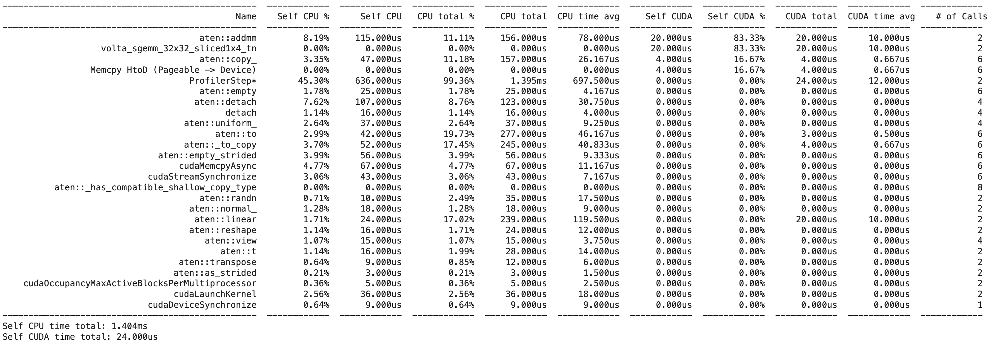
However, we also get a Chrome trace file that we can open in Chrome to visualize the profiling data:
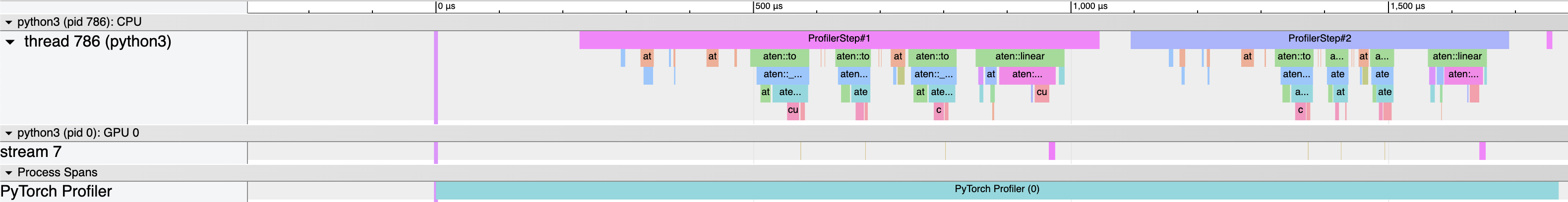
We can see that the majority of the time is actually spent on the cpu, moving data to the GPU, whereas the actual matrix multiplication is quite fast (and uses a special CUDA kernel called volta_sgemm_32x32_sliced1x4_tn).
1.4 ncu profiler
The ncu profiler is a command-line tool that comes with the CUDA toolkit. It is a very powerful tool that allows you to profile your CUDA kernels in great detail. You invoke it by running ncu python script.py. It will then run your script and profile all the CUDA kernels that are called. It will then generate a report in the form of a ncu_logs file that contains helpful numbers and recommendations on how to optimize your code.
A similar tool from the CUDA toolkit is nsys, which also allows you to profile your code. It is however less focused on detailed CUDA kernel performance analysis, but more the overall system-wide performance, as well as understanding how the communication between CPU and GPU impacts performance.
We can mark code we want to profile via the torch.cuda.nvtx API that allows us to start capturing via range_push() and stop capturing via range_pop(). In the code example below, we profile a single linear layer; we also delay tehs tart of profiling until iteration 10 to allow for warm-up time.
import torch
import torch.nn as nn
import torch.nn.functional as F

for i in range(20):
    if i == 10: torch.cuda.cudart().cudaProfilerStart()
    if i >= 10: torch.cuda.nvtx.range_push(f"Iteration {i}")
    data = torch.randn(1, 1, 32, 32).cuda()
    output = torch.nn.Linear(32, 32).cuda()(data)
    if i >= 10: torch.cuda.nvtx.range_pop()
The call to torch.cuda.cudart().cudaProfilerStart() indicates to NSys to only care about profiling from this iteration on.
To get the profiling output now, we need to install and use the nsys toolkit. There are many CLI options you can choose for it, but one of the simplest calls might be nsys profile -o output_profile python script.py. This will produce a file called output_profile.nsys-rep which you can then open in the NSight Systems UI (if you run your profiling on a remote machine, transfer the report file your local machine so that you can run the GUI application). For the a simple linear layer it will look something like this:
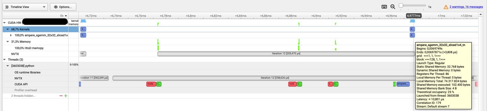
NSys Profiling report for a single linear layer in PyTorch.
We can see that the actual computation only takes a bit of time, while there is a long time before that gets spent on data transfer via calls to the CUDA API like MemCopy. Only at the end is the ampere_sgemm_32x32_sliced kernel called that performs the actual matrix multiplication in tiles of 32 by 32.
To profile more complex code like a whole ResNet for example, we can either set the profiling points still manually as described in this community post or we can use tools such as autonvtx that just wrap our model and deal with the profiling setup for us. Doing this for a simple ResNet results in the following profiler output:
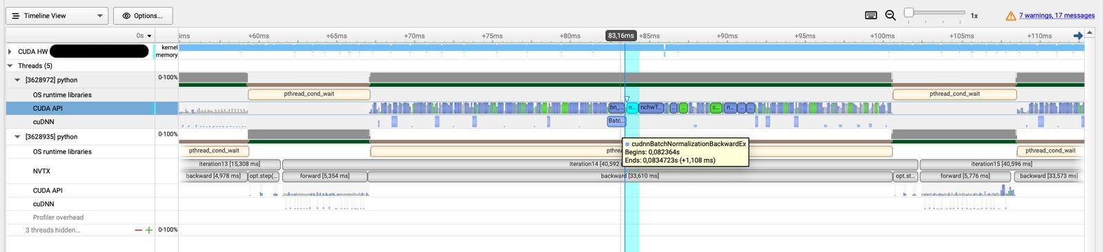
NSys Profiling report for a ResnNet in PyTorch.
In this case we can see that a way bigger chunck of time is spent on CUDA calls and actual computation. We also see that there are calls to the cuDNN backend for operations such as batch normalization.
NSys can seem overwhelming and is a bit more overhead to get set up compared to the options presented before, but it can give you some detailed insights as well as suggestions what kind of things to improve in your code.
2. Integrating CUDA kernels into PyTorch
CUDA is written in C++ and is a parallel computing platform and application programming interface (API) model created by Nvidia. It allows software developers to use a CUDA-enabled graphics processing unit (GPU) for general purpose processing. Since it is written in C++, it is not immediatly obvious how to integrate it into our ML code that is normally written in Python libraries like PyTorch. However, there are several options.
2.1 load_inline function
The easiest way to integrate CUDA kernels into PyTorch is to use the torch.utils.cpp_extension module. This module allows you to compile C++ code into a shared library and then load it into Python. Here is an example of how to do this via the load_inline function for a simple matrix squaring operation:
import torch
from torch.utils.cpp_extension import load_inline

# Define the CUDA kernel and C++ wrapper
cuda_source = '''
__global__ void square_matrix_kernel(const float* matrix, float* result, int width, int height) {
    int row = blockIdx.y * blockDim.y + threadIdx.y;
    int col = blockIdx.x * blockDim.x + threadIdx.x;

    if (row < height && col < width) {
        int idx = row * width + col;
        result[idx] = matrix[idx] * matrix[idx];
    }
}

torch::Tensor square_matrix(torch::Tensor matrix) {
    const auto height = matrix.size(0);
    const auto width = matrix.size(1);

    auto result = torch::empty_like(matrix);

    dim3 threads_per_block(16, 16);
    dim3 number_of_blocks((width + threads_per_block.x - 1) / threads_per_block.x,
                          (height + threads_per_block.y - 1) / threads_per_block.y);

    square_matrix_kernel<<<number_of_blocks, threads_per_block>>>(
        matrix.data_ptr<float>(), result.data_ptr<float>(), width, height);

    return result;
    }
'''

cpp_source = "torch::Tensor square_matrix(torch::Tensor matrix);"

# Load the CUDA kernel as a PyTorch extension
square_matrix_extension = load_inline(
    name='square_matrix_extension',
    cpp_sources=cpp_source,
    cuda_sources=cuda_source,
    functions=['square_matrix'],
    with_cuda=True,
    extra_cuda_cflags=["-O2"],
    # build_directory='./load_inline_cuda',
    # extra_cuda_cflags=['--expt-relaxed-constexpr']
)

a = torch.tensor([[1., 2., 3.], [4., 5., 6.]], device='cuda')
print(square_matrix_extension.square_matrix(a))

# Output:
# tensor([[ 1.,  4.,  9.],
#         [16., 25., 36.]], device='cuda:0')
We see that the output is the same as if we used a PyTorch function. If we want to inspect the generated code, we can set the build_directory argument of the load_inline function to see the generated code in the specified directory.
2.2 Numba
Another way to integrate CUDA kernels into PyTorch is to use the numba library. This is a just-in-time (JIT) compiler that translates Python functions to optimized machine code at runtime using the industry-standard LLVM compiler library. It can also be used to generate CUDA kernels.
from numba import cuda

# CUDA kernel
@cuda.jit
def square_matrix_kernel(matrix, result):
    # Calculate the row and column index for each thread
    row, col = cuda.grid(2)

    # Check if the thread's indices are within the bounds of the matrix
    if row < matrix.shape[0] and col < matrix.shape[1]:
        # Perform the square operation
        result[row, col] = matrix[row, col] ** 2

# Example usage
import numpy as np

# Create a sample matrix
matrix = np.array([[1, 2, 3], [4, 5, 6]], dtype=np.float32)

# Allocate memory on the device
d_matrix = cuda.to_device(matrix)
d_result = cuda.device_array(matrix.shape, dtype=np.float32)

# Configure the blocks
threads_per_block = (16, 16)
blocks_per_grid_x = int(np.ceil(matrix.shape[0] / threads_per_block[0]))
blocks_per_grid_y = int(np.ceil(matrix.shape[1] / threads_per_block[1]))
blocks_per_grid = (blocks_per_grid_x, blocks_per_grid_y)

# Launch the kernel
square_matrix_kernel[blocks_per_grid, threads_per_block](d_matrix, d_result)

# Copy the result back to the host
result = d_result.copy_to_host()

# Result is now in 'result' array
print(matrix)
print(result)
3. Integrate Triton kernels into PyTorch
3.1 Using Triton
Triton is both a domain-specific language (DSL) and a compiler for writing highly efficient GPU code. It actually does not generate CUDA code, but PTX code, which is a lower-level intermediate representation of the CUDA code (basically the assembly language of CUDA). Newer features in PyTorch like torch.compile actually leverage Triton kernels under the hood, so it is worth understanding how it works. Since Triton is written in Python, it is easy to integrate with PyTorch. Here is an example of how to use Triton to write a simple matrix squaring operation:
# Adapted straight from https://triton-lang.org/main/getting-started/tutorials/02-fused-softmax.html
import triton
import triton.language as tl
import torch

@triton.jit
def square_kernel(output_ptr, input_ptr, input_row_stride, output_row_stride, n_cols, BLOCK_SIZE: tl.constexpr):
    # The rows of the softmax are independent, so we parallelize across those
    row_idx = tl.program_id(0)
    # The stride represents how much we need to increase the pointer to advance 1 row
    row_start_ptr = input_ptr + row_idx * input_row_stride
    # The block size is the next power of two greater than n_cols, so we can fit each
    # row in a single block
    col_offsets = tl.arange(0, BLOCK_SIZE)
    input_ptrs = row_start_ptr + col_offsets
    # Load the row into SRAM, using a mask since BLOCK_SIZE may be > than n_cols
    row = tl.load(input_ptrs, mask=col_offsets < n_cols, other=-float('inf'))

    square_output = row * row

    # Write back output to DRAM
    output_row_start_ptr = output_ptr + row_idx * output_row_stride
    output_ptrs = output_row_start_ptr + col_offsets
    tl.store(output_ptrs, square_output, mask=col_offsets < n_cols)


def square(x):
    n_rows, n_cols = x.shape
    # The block size is the smallest power of two greater than the number of columns in x
    BLOCK_SIZE = triton.next_power_of_2(n_cols)
    # Another trick we can use is to ask the compiler to use more threads per row by
    # increasing the number of warps (num_warps) over which each row is distributed.
    # You will see in the next tutorial how to auto-tune this value in a more natural
    # way so you don't have to come up with manual heuristics yourself.
    num_warps = 4
    if BLOCK_SIZE >= 2048:
        num_warps = 8
    if BLOCK_SIZE >= 4096:
        num_warps = 16
    # Allocate output
    y = torch.empty_like(x)
    # Enqueue kernel. The 1D launch grid is simple: we have one kernel instance per row o
    # f the input matrix
    square_kernel[(n_rows, )](
        y,
        x,
        x.stride(0),
        y.stride(0),
        n_cols,
        num_warps=num_warps,
        BLOCK_SIZE=BLOCK_SIZE,
    )
    return y


torch.manual_seed(0)
x = torch.randn(1823, 781, device='cuda')
y_triton = square(x)
y_torch = torch.square(x)
assert torch.allclose(y_triton, y_torch), (y_triton, y_torch)
We see that the output of the Triton kernel is the same as the output of the PyTorch function.
3.2 Debugging Triton
Once we go to compiled code, we hopefully gain speed, but loose some of the flexibility that comes with eager execution, e.g. easy debugging via pdb and other Python debuggers or simple print statements.
Fortunately, Triton has a debugger now: we can invoke it by changing the triton.jit decorator to triton.jit(interpret=True). This will allow you to set normal Python breakpoints and step through the kernel line by line.
The interpret=True option was recently deprecated, so you can instead use os.environ["TRITON_INTERPRET"] = "1".
When doing that, you will see that most objects in the kernel are of the type WrappedTensor. So if you want to inspect a variable, you have to access its .tensor attribute.
Let’s look at this in action with a simple vector addition kernel from the Triton Docs.
If you do not have a GPU available, you can run this code in a Google Colab by first choosing a GPU runtime and then executing the following lines to get the latest Triton version and set up your CUDA libraries correctly:
!ldconfig /usr/lib64-nvidia!ldconfig -p | grep libcud!pip install -U --index-url https://aiinfra.pkgs.visualstudio.com/PublicPackages/_packaging/Triton-Nightly/pypi/simple/ triton-nightly
Let us implement a simple vector addition kernel together with a helper function to call the kernel as well as some code to generate data and call that function:
import triton
import triton.language as tl
import torch

@triton.jit
def add_kernel(x_ptr, y_ptr, output_ptr, n_elements, BLOCK_SIZE: tl.constexpr):
    pid = tl.program_id(axis=0)
    breakpoint()
    block_start = pid * BLOCK_SIZE
    offsets = block_start + tl.arange(0, BLOCK_SIZE)
    mask = offsets < n_elements
    x = tl.load(x_ptr + offsets, mask=mask)
    y = tl.load(y_ptr + offsets, mask=mask)
    output = x + y
    tl.store(output_ptr + offsets, output, mask=mask)

def add(x: torch.Tensor, y: torch.Tensor):
    output = torch.empty_like(x)
    assert x.is_cuda and y.is_cuda and output.is_cuda
    n_elements = output.numel()
    grid = lambda meta: (triton.cdiv(n_elements, meta['BLOCK_SIZE']), )
    add_kernel[grid](x, y, output, n_elements, BLOCK_SIZE=1024)
    torch.cuda.synchronize()
    return output

torch.manual_seed(0)
size = 98432
x = torch.rand(size, device='cuda')
y = torch.rand(size, device='cuda')
output_torch = x + y
output_triton = add(x, y)
print(f'The maximum difference between torch and triton is '
      f'{torch.max(torch.abs(output_torch - output_triton))}')
Does not seem to complicated, but what are all these in-built Triton variables like tl.program_id? What do the offsets look like? And what values do my data pointers have? If we try to set breakpoint() to enter the PDB debugger, we get a NameError.
To answer these questions, import os and set the interpret flag for Triton to true: os.environ["TRITON_INTERPRET"] = "1". Now our breakpoint() works like a charm and we can interactively debug our Triton kernel (even inside a notebook!).
Via this, we learn for example that our pid is 0 in the first iteration, 1 in the second and so on! These iterations correspond to the workgroup/tile id, similar to the blockIdx in CUDA.
We also see that the offsets are a contiguous array of indices that are used to later access the vectors. We can also see that x_ptr and y_ptr contain memory addresses. So what happens is that in x = tl.load(x_ptr + offsets, mask=mask), Triton loads the whole block of memory from x_ptr and including all the offset locations. The compiler here makes sure that these memory accesses are efficient via e.g. memory coalesence.
3.3 Triton Deep-Dive
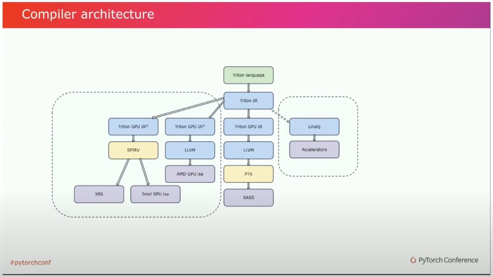
What does Triton do under the hood? It converts the Python code first into a custom Triton IR and then via the Triton compiler into the well-known LLVM-IR. From there PTX code is generated. Basically, Triton leverages LLVM heavily and (quote from the paper) “just a few data- and control-flow extensions to LLVM-IR could enable various tile-level optimization passes which jointly lead to performance on-par with vendor libraries.” These extensions allow Triton to do things like shared memory allocation or memory coalescence, things that in CUDA the GPU programmer has to handle manually.
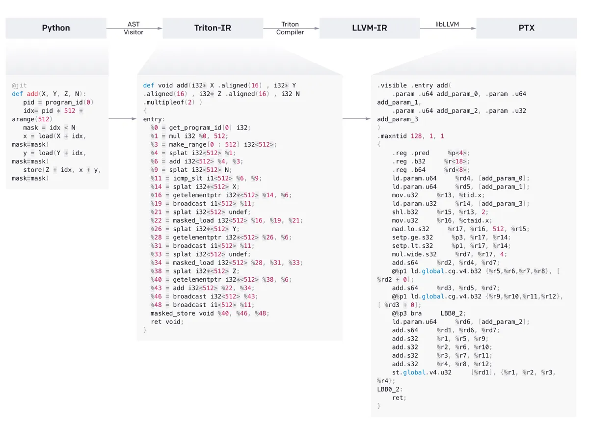
From this news article
We can look at all these different intermediate representations by saving the compiled kernell to a variable and then accessing the asm field that contains the IRs for various levels.
compiled = add_kernel[grid](x, y, output, n_elements, BLOCK_SIZE=1024)
print("IR", compiled.asm['ttir'])
print("TTGIR", compiled.asm['ttgir'])
print("LLIR", compiled.asm['llir'])
print("PTX", compiled.asm['ptx'])
- TTIR (Intermediate Representation): This IR is what people generally refer to when they say Triton IR. Inspecting it you see that it looks relatively similar to the original Triton code, just with many of the operations split up into more fundamental steps like initialising constants, loading and broadcasting data and finally (after computation) storing it again. We see that our original kernel is now wrapped in an
IR moduleas att.func public @kernel_name. - TTGIR (Triton Thread-Group Intermediate Representation): Triton can be used for different accelerators, and the GPU is one of them. In that case, Triton will lower TTIR into TTGIR, where GPU-specific operations like thread synchronizations, call coalescences and shared memory allocations are performed.
- LLIR (Low-Level Intermediate Representation): After TTGIR, the code is transformed into LLIR, the lowest level of IR. If we inspec the LLIR, we can see at the start the we use a
LLVMDialectModule. This indicates that the IR we are talking about is the LLVM IR, part of a larger collections of module and reusable compiler technologies as part of the LLVM project. The idea is that no matter from which IR we lower into LLVM, we can use this IR to translate the code into different backends (for example into machine code for NVIDIA or AMD GPUs). The fact that we use aLLVMDialectModulehints that we do not only leverage LLVM, but the dialect part hints at the use of MLIR, a successor project that tries to unify the toolset of not only the IR to backend process, but also the toolset to create these IRs in the first place. You can read more about MLIR in the original paper, this developer presentation or this blogpost. - PTX (Parallel Thread Execution, also NVPTX): PTX is now the ISA (instruction set architecture) used in NVIDIA GPUs. If we normally write CUDA kernels, the NVCC compiler translates CUDA C++ code into PTX; here, Triton ends up at the same destination via a different route passing Triton IR and LLVM IR. PTX is now a proper assembly language represented in ASCII text specific for NVIDIA GPUs that contain compilers in their graphic drivers to the assembly language SASS, which is specific for each different graphics card to enable device-specific optimisations. This code is then finally transformed into binary code and executed by the GPU.
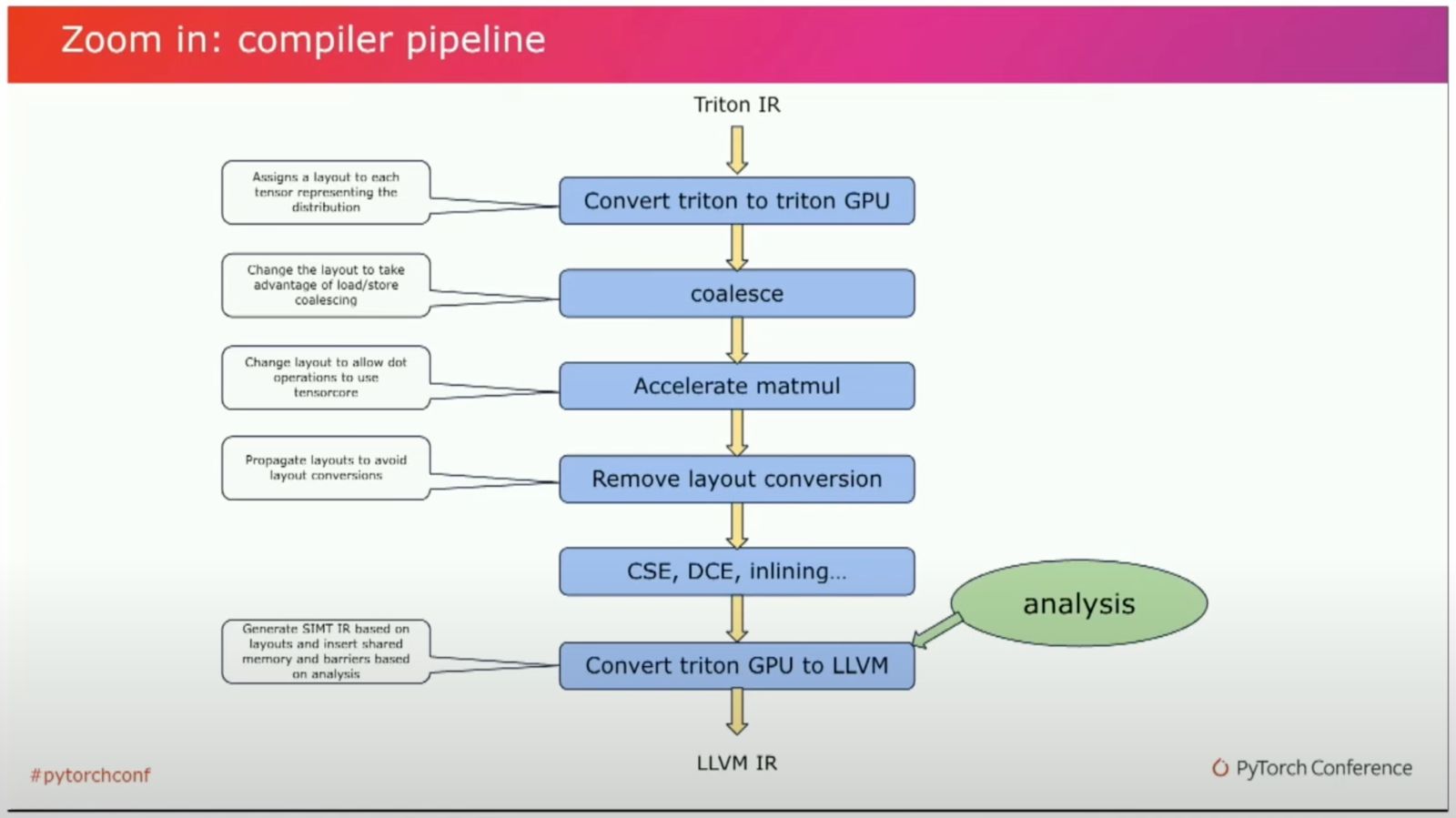
Triton Compiler Pipeline (Link)
Looking at the Triton Compiler Pipeline from Triton IR to LLVM IR, we see that many of the optimizations we specify in CUDA are performed in this transformation process; for example memory coalescence, matmul acceleration and layout adaptions.
The interesting part about Triton is that it is not limited to a specific set of hardware architectures, but can in principle be used for a variety of ISAs (Instruction Set Architectures).
Triton Compiler Ecosystem (Link)
While most programs targeted for GPUs will probably end up in LLVM IR and then get translated into the vendor-specific ISAs, code for CPUs, FPGAs and other hardware can get translated into other compiler backends, making the ecosystem modular.
3.4 Benchmarking Triton
We want to benchmark our Triton kernels similar to our CUDA kernels, of course; if they do not give us speed-ups we would not have needed to deal with them in the first place!
For profiling, we use the decorator triton.testing.perf_report to get a performance report of our kernel.
@triton.testing.perf_report(
        triton.testing.Benchmark(
            x_names=['size'],
            x_vals=[2**i for i in range(12, 28, 1)],
            x_log=True,
            line_arg='provider',
            line_vals=['triton', 'torch'],
            line_names=['Triton', 'Torch'],
            styles=[('blue', '-'), ('green', '-')],  # Line styles.
            ylabel='GB/s',  # Label name for the y-axis.
            plot_name='matrix-square-performance',  # Name for the plot. Used also as a file name for saving the plot.
            args={},  # Values for function arguments not in x_names and y_name.
        ))

def benchmark(size, provider):
    x = torch.rand(size, device='cuda', dtype=torch.float32)
    quantiles = [0.5, 0.2, 0.8]
    if provider == 'torch':
        ms, min_ms, max_ms = triton.testing.do_bench(lambda: x**2, quantiles = quantiles)
    if provider == 'triton':
        ms, min_ms, max_ms = triton.testing.do_bench(lambda: square(x), quantiles=quantiles)
    gbps = lambda ms: 12 * size / ms * 1e-6
    return gbps(ms), gbps(max_ms), gbps(min_ms)

benchmark.run(show_plots=True, print_data=True)
With this benchmark, we get both a print-out of our data as well as a graphical representation.
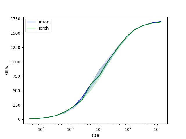
Triton benchmark plot.
We can see that in this case, there is no significant speed-up over PyTorch; however looking at more complex examples on the Triton page, there are speed-ups to be achieved.
To read more about Triton, you can have a look at the original research paper, a video by the author Philippe Tillet and a Reddit discussion where he himself gave some useful perspectives on the project.
4. torch.compile
To get a feel for how Triton fits into the PyTorch2 compilation stack, we can leverage the fact that torch.compile actually uses Triton under the hood. We can just write a simple function and then call torch.compile on it. Then, when running the script, we set the environment variable os.environ["TORCH_LOGS"] to different values (depending on which stage of the PyTorch compilation process we want to investigate) or set these values directly in PyTorch via torch._logging.set_logs(argument) with different arguments.
| Stage | Value for TORCH_LOGS (Env. variable) | Argument to set_logs(Python function) |
|---|---|---|
| Dynamo Tracing | +dynamo | dynamo=logging.DEBUG |
| Traced Graph | graph | graph=True |
| Fusion Detections | fusion | fusion=True |
| Triton Output Code | output_code | output_code=True |
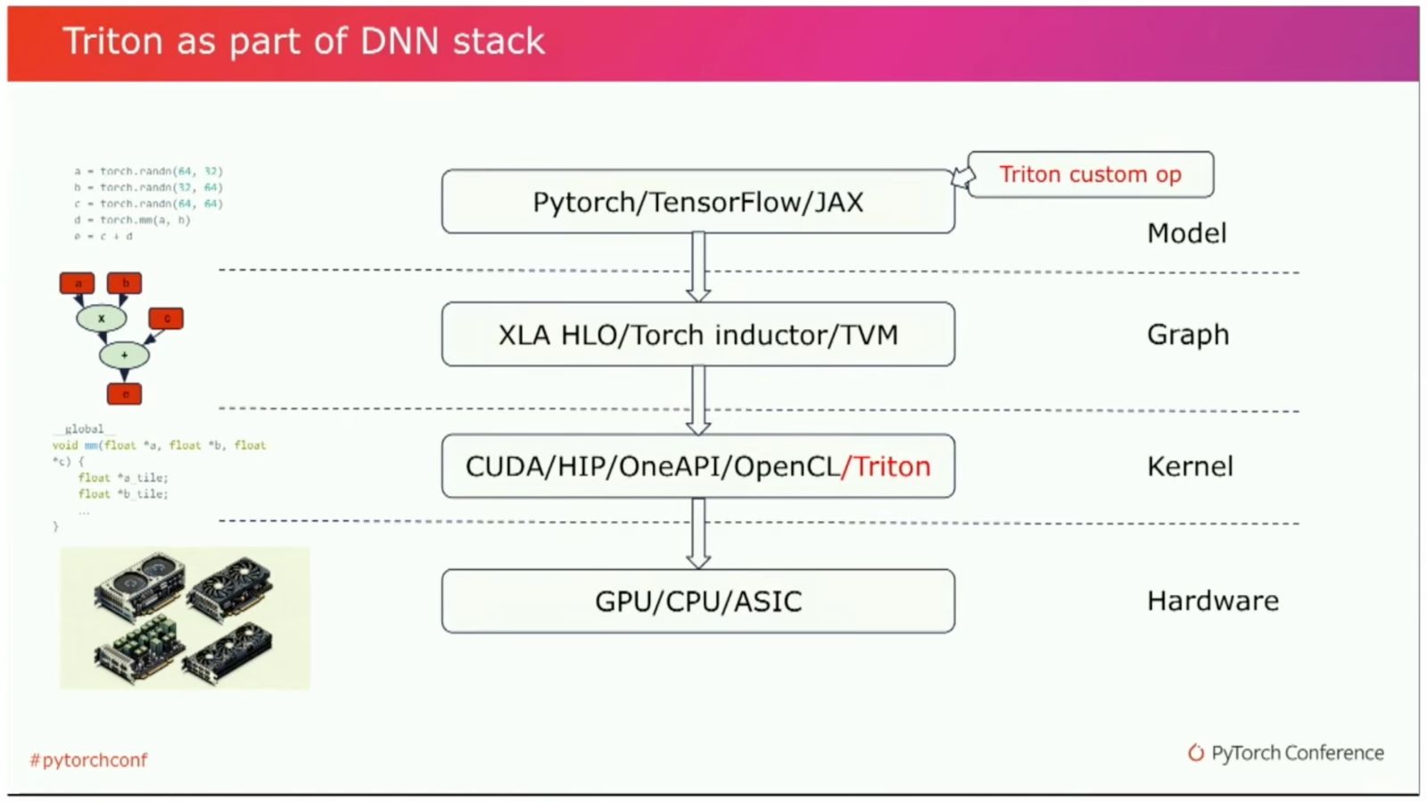
Triton DL Stack (Link)
Looking at this, we can see that Triton leverages some heuristics to enable autotuning and other efficiency improvements. For example, it infers data types and element numbers and then uses this information to optimize the kernel.
Credits
Thanks to the CUDA MODE lecture series for the inspiration for this post and the community around that for interesting discussions!