Dealing with the flood of protein structures

07 Apr 2024 in Proteins

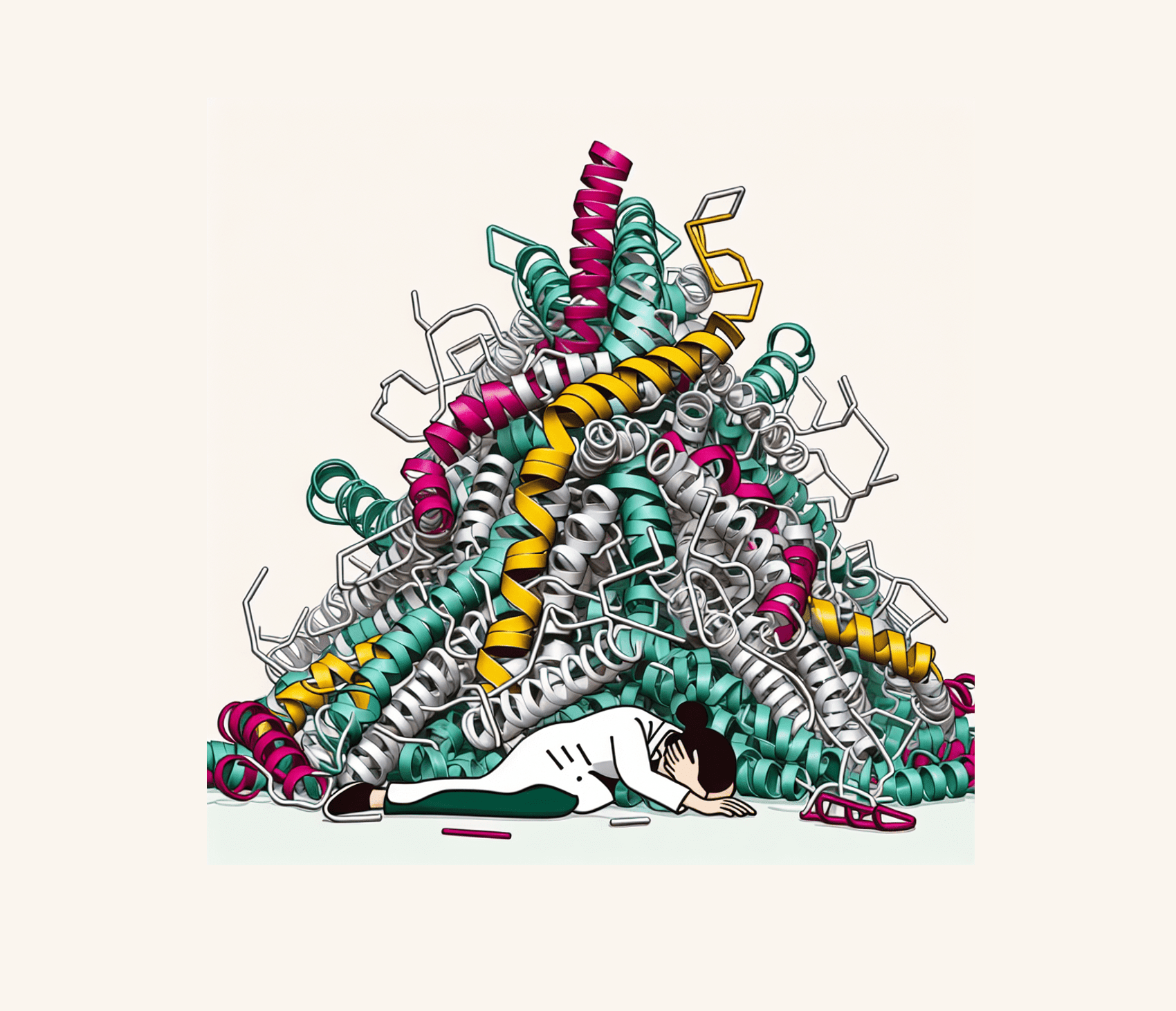
How structure prediction changed the questions we ask and the tools we use

With the explosion of protein structure prediction and the sheer number of predicted protein structures available in databases nowadays, we can ask exciting new questions that would have been unanswerable only a few years ago. However, we need new tools in order to answer these questions and deal with the flood of structural data. In this post, I describe a few of these new tools and the reasoning behind them.

How protein structure prediction changed the game
FoldComp: compressing protein structures to managable sizes
MMseqs2: sequence alignment in speed-mode
FoldSeek: structural clustering of the protein universe
Applications: clustering the protein universe

How protein structure prediction changed the game

The PDB as a database of experimental protein structures keeps growing, currently standing at nearly 218k entries. However, it seems small compared to the AlphaFoldDB (>200m) and ESMAtlas (772m structures), powered by the recent advances in protein structure prediction via methods like AlphaFold2 and ESMFold.

This development changed the game in protein biology. While until recently the gap between available protein sequences and structures widened further and further, we suddenly have a wealth of structural information that was unimaginable a decade ago. This quote from Mohammed AlQuraishi (Columbia University) sums up this paradigm shift well:

Everything we did with protein sequences we can now do with protein structures

While that is a theoretically true and very exciting prospect, there is one big problem: we do not have tools to deal with such amounts of structural data. Here a visual comparison between the size of the PDB and the AFDB:

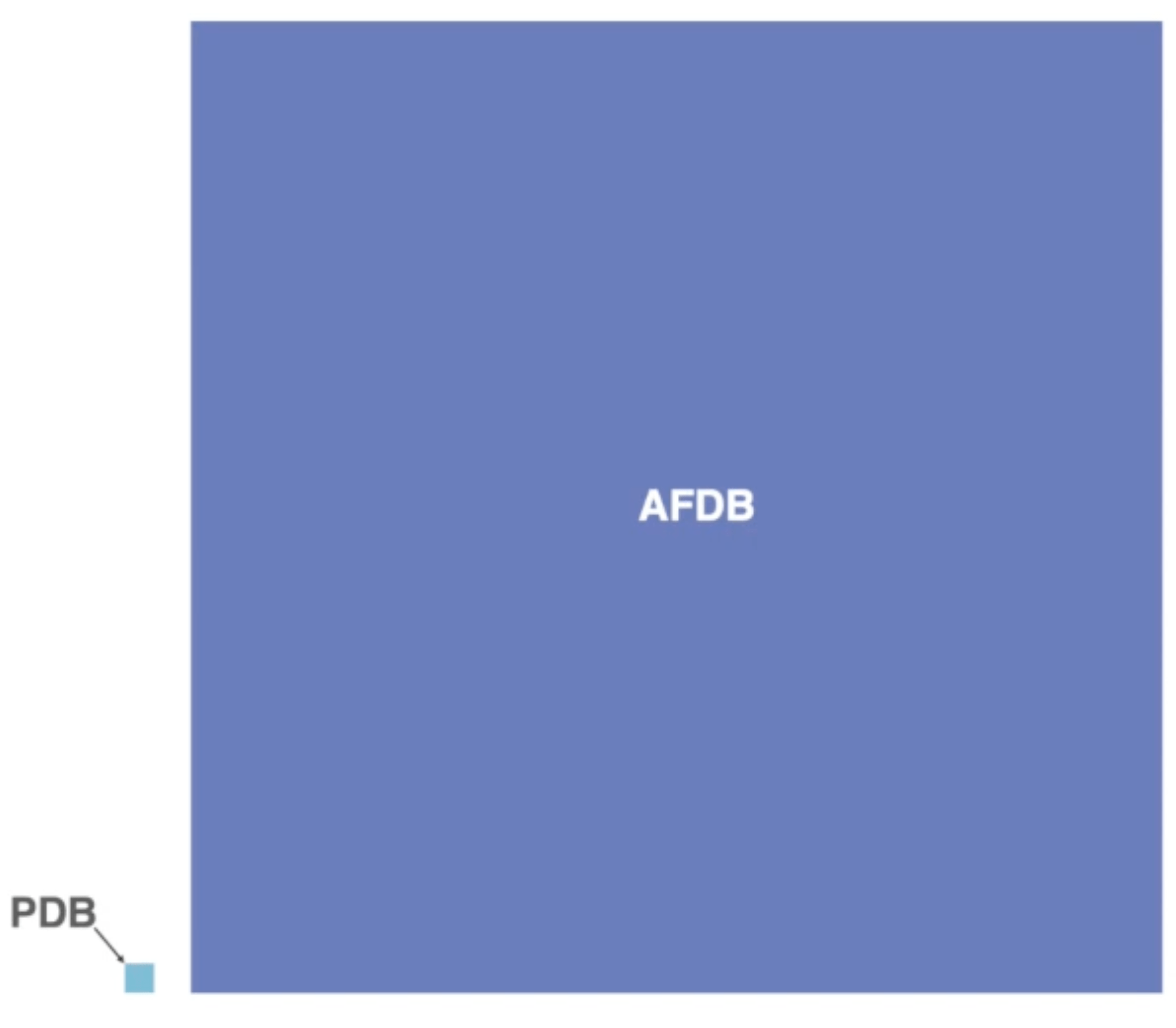
Visual comparison of the size of the PDB vs the AFDB. Source: YouTube

You can see that we deal with a different order of magnitude in data here. This brings up a plethora of issues, starting from pure memory usage (the storage for AFDB is 23 TB) to questions of how we move these enormous amounts of data and also process them.

Many groups have developed tools in the last years to tackle this issue. Especially the Steinegger lab has produced some fantastic tools in that space from which I want to present three here in this blogpost: Foldcomp for structure compression, Foldseek for structure clustering and mmseqs for sequence clustering (also very important in that context for generating both input MSAs and training splits).

steinegger_tools

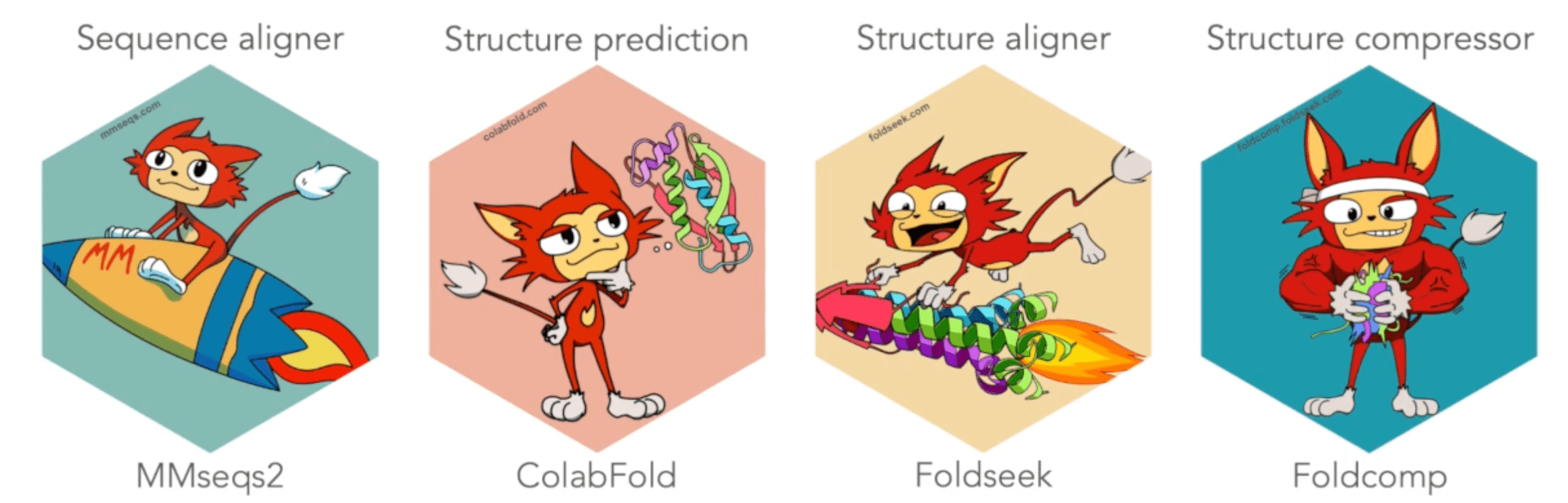
Tools from the Steinegger Lab. Source: YouTube

FoldComp: compressing protein structures to managable sizes

Paper
Talk
The trouble with compression

A perfect compression format satisfied all these three conditions:

The compressed files are small.
The compression and decompression algorithms are fast
The reconstruction is either lossless or (if lossy) has minimal reconstruction error.

Fulfilling all of these at the same time is hard, so one always has to think about how to balance between them.

As described in the first section of this post, there have been efforts for compressed protein structure formats such as MMTF or binaryCIF. However, given the sheer amount of predicted protein structures, the authors decided that more efficient algorithms are needed.

People have tried this in the past by talking inspiration from image compression algorithms such as PNG and JPEG as in the example of the PIC algorithm. These lossless formats are great since they reconstruct your data perfectly, but often leave some performance in terms of both speed and size on the table by focusing on reconstruction quality.

Therefore, looking into lossy compression formats often pays off if you are fine with paying a small penalty in terms of reconstruction error. Since our measurements of protein structures contain measurement errors anyway, we can often pay this penalty and still get great results for our biological problems such as for example energy calculations from MD trajectories.

The FoldComp compression scheme

In this spirit, Kim et al. from the Steinegger lab decided to build a lossy compression format that converts the nearly 100 bytes of 3D coordinates per residue into only 13 bytes of compressed internal coordinates (in this case torsion angles).

FoldComp

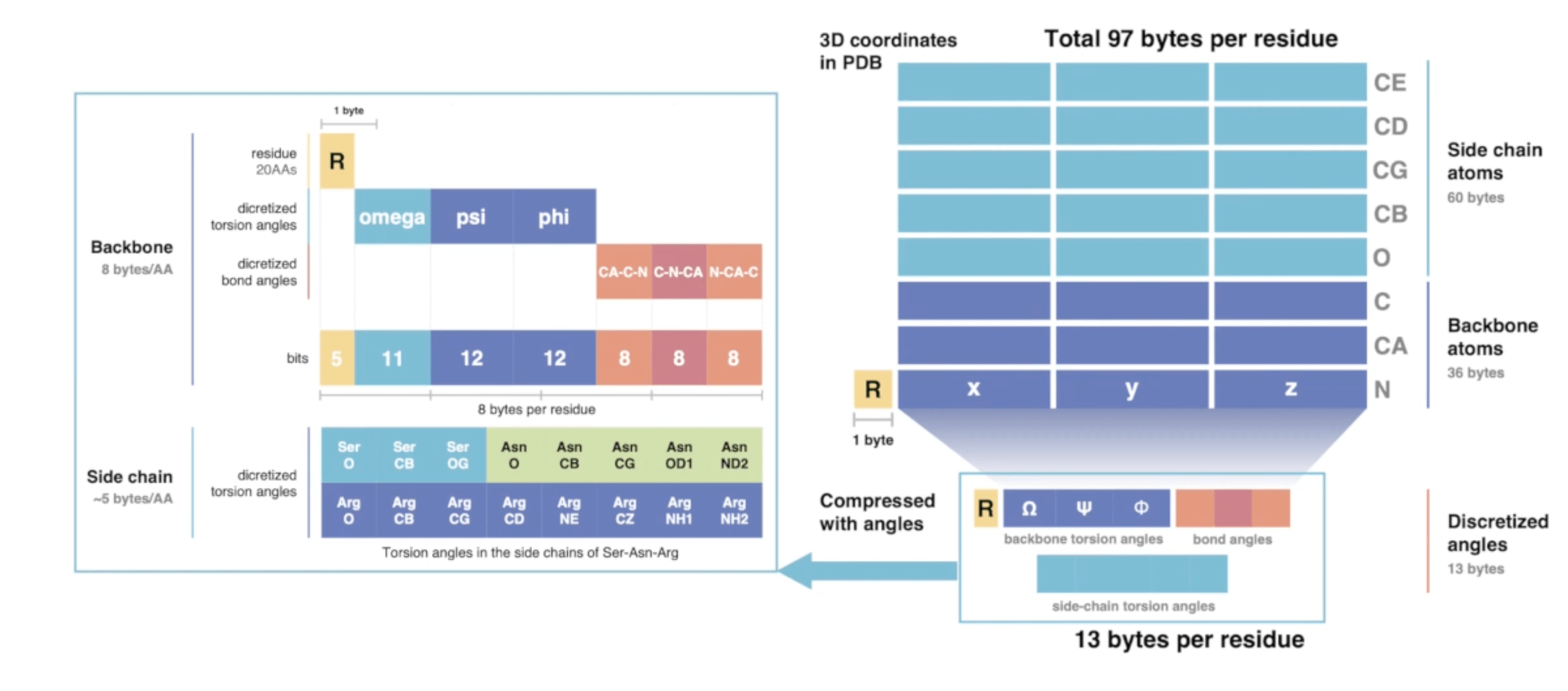
FoldComp compression scheme. Source: YouTube

As you can see in that graphic, they do not only save the backbone and side-chain torsion angles, but also bond angles. This should in theory not be necessary since one should be able to reconstruct the full-atom structure by just using torsion angles. However, this theory assumes an idealised protein backbone geometry with constant bond angles, which is a bit too simplistic in practice to get very low reconstruction error. Encoding these bond angles improves the reconstruction a lot.

In order to not make the space occupied by both torsion and bond angles to demanding, they employ a quantisation step where they save both of these entities as discretised pre-defined values. This procedure is also commonly known as binning and has been used to great extent machine learning for weights and activations as well as for optimiser states, up to the extreme of recent 1-bit LLMs.

NeRF and the lever-arm effect

Saving the actual bond angles helped to lower the reconstruction error for the first few residues that were reconstructed. However, the longer the polymer chain get, the bigger the reconstruction error became down the line. This problem is related to a phenomenon known as lever-arm effect in engineering. It describes the propagation of an error on the rotation measurement in a series of successive measurements, with the error magnitude increasing the longer the distance between the original measurement and the reconstruction.

To understand this in the context of proteins, let’s look at the method FoldComp and others in the field use to convert the stored torsion angles back into 3D coordinates: the NeRF (Natural Extension Reference Frame) method (unrelated to the NeRF in machine learning which stands for Neural Radiance Fields).

There have been multiple versions of NeRF such as pNeRF and MP-NeRF that make it more efficient via parallelisation, but the basic algorithmic ideas stay the same:

We can place our first backbone atom wherever we want and define this as our origin: $A_1(0,0,0)$
Given a first backbone atom ( $A_1$ ), we can place the second one arbitrarily in space and just constrain its position by the known bond distance $d_1$ : $A_2(0,0,d_1)$
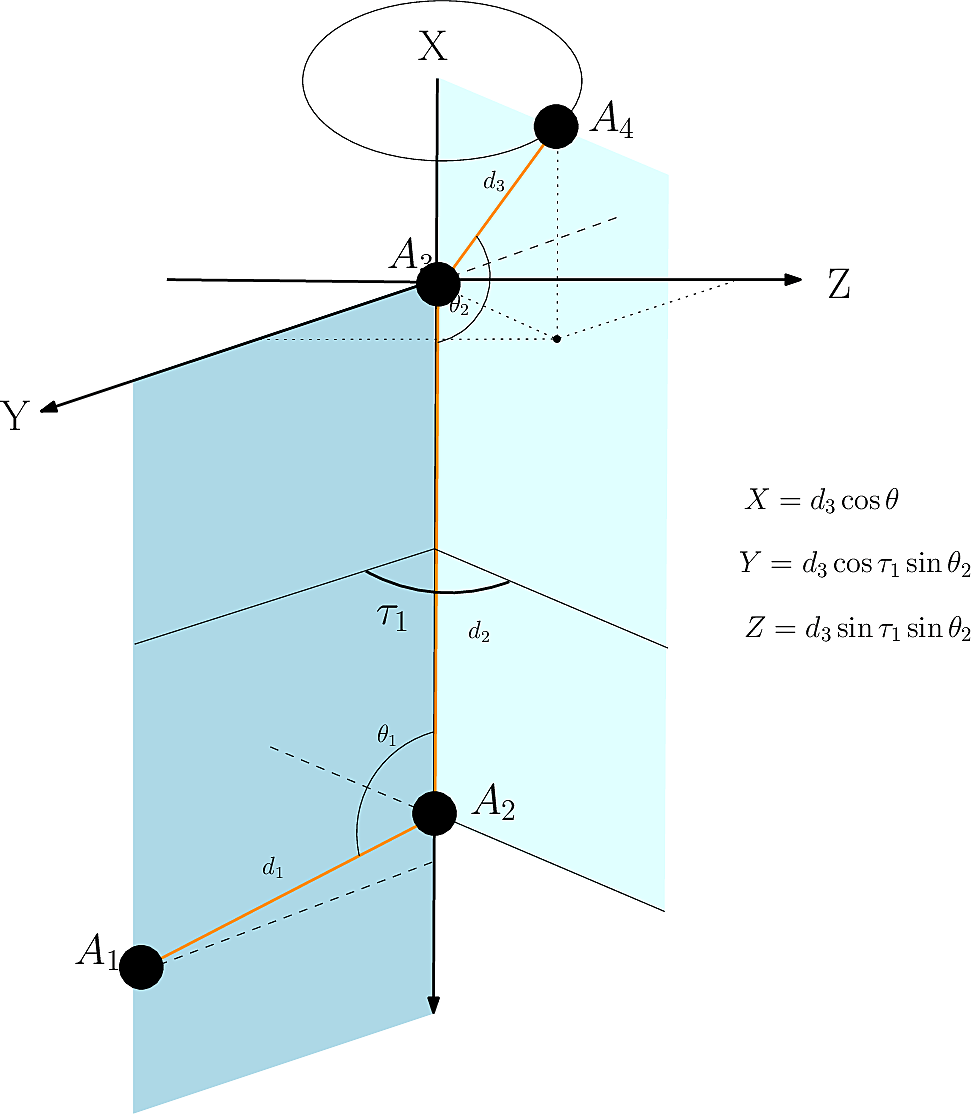
Given the first two backbone atoms ( $A_1, A_2$ ), we can place the third one in space by using the literature bond distance $d_2$ and angle $\theta_1$ : $A_3(0, \sin(\theta_1) * d_2, d1 - \cos(\theta_1) * d_2)$
Given the first three backbone atoms ( $A_1, A_2, A_3$ ), we can place the fourth one in space by using the literature bond distance ( $d_3$ ), the literature (or saved in the case of FoldComp) angle $\theta_2$ and the stored torsion angle $\tau_1$ . To do this, we first define a new coordinate system called specialised reference frame centered at $A_3$ using spherical coordinates and places $A_4^*$ there:

\begin{aligned} %!!15 A_4^* &= (d_3 \cos(\theta_2), d_3 \cos(\tau_1) \sin(\theta_2), d_3 \sin(\tau_1) \sin(\theta_2)) \end{aligned}

Calculation of $A_4^*$ in the specialised reference frame.

We then rototranslate $A_4^*$ back from that specialised reference frame back to our original coordinate system via $A_4 = RA_4^* + A_3$ and with $\begin{aligned} %!!15 R &= [\hat{A}_{2-3}, \hat{n} \times \hat{A}_{2-3}, \hat{n}] \\ \hat{A}_{2-3} &= \frac{A_2 A_3}{\mid A_2 A_3 \mid}\\ \hat{n} &= \frac{A_1 A_2 \times \hat{A}_{2-3}}{\mid A_1 A_2 \cross \hat{A}_{2-3} \mid } \end{aligned}$

Rototranslation of $A_4^*$ back to the original coordinate system to form $A_4$ .

We can repeat step 4 for all forthcoming atoms until we are at the end of the polymer chains.

Reconstruction of the backbone works in a similar way, just using different values for bond distances, bond angles and torsion angles.

NeRF algorithm. Source: Structural Bioinformatics Library

As a fun fact, and another anecdote to how small the world of science is: Charlie Strauss, the lead author of the original NeRF paper from 2005, is from Seattle and did a summer job as a highschooler with Prof Tillman at the University of Washington working on mars metereology. That gave him both inspiration and grit to go into science, ending up in the Los Alamos National Laboratory where he supervised the NeRF paper that was published in 2005. As another unexpected twist of events, in the 90s he took a year long sabbatical at UW working in the lab of David Baker and improving their Rosetta algortihm for protein structure prediction. Yes, you heard right, the David Baker whose lab became synonymous with protein design and is still a pioneer in that field. Wha a funny world we live in.

Now with this NeRF algorithm at hand, we can go about reconstruction our 3D cartesian coordinates from our internal coordinates represented as torsion and bond angles. There is only one problem: the previously mentioned lever-arm effect.

We will get pretty accurate reconstruction for the first few residues, but small errors will accumulate since every reconstruction step is only relative to the previous ones. You can imagine this with an analogy: let’s say you want to follow a route on Google Maps. The routing instructions are successive relative statements (“turn left in 100 meters”, “go straight for 1km”, …), similar to how the torsion and bond angles during NeRF reconstruction are relative reconstruction steps. What you want in the end however is the full path to your correct destination; you are therefore “reconstructing” the correct path from these relative instructions.

Now if you follow the instructions very carefully at the start and only turn left instead of right close to the destination you will still be very close to your actual destination; your reconstruction error is low. However, if you start off your journey by taking the wrong exit in a roundabout and just keep following the instructions (ignoring that Google Maps will try to course-correct you), you will end up god-knows where! The error you made at the beginning propagates down to all of your successive steps and will accumulate, leading to a massive reconstruction error at the end.

The same is happening for the NeRF algorithm: a small reconstruction error at the start will lead to a large reconstruction error later along the peptide backbone, leaving you with a poorly reconstructed protein.

This phenomenon is not new by any means, not even in the protein community: while the first protein structure predicition methods like RGN used recurrent networks based on torsion angle prediction for reconstructing protein backbones, later methods like AlphaFold2 instead leveraged transformer-based architectures that utilise parallel reconstruction directly in Cartesion space instead of sequential reconstruction via internal coordinates. Similar observations where made in protein structure generation: FoldingDiff, a diffusion model by Microsoft Research, leveraged a torsion-angle based representation to generate protein backbones, and while that worked well for relatively short proteins, they note on page 4 of the SI that for larger proteins lever-arm effects play a role (although the model seems to be relatively robust in some cases).

The lever-arm solution: bidirectional NeRF and anchoring

While some machine learning algorithms like Int2Cart were developed to ameliorate the lever-arm problem, the FoldComp authors decided to stick with good-old NeRF and instead give it a boost via two approaches:

Bidirectionality: They start NeRF from the N- and the C-terminus of the polypeptide chain and using a weighted average of both reconstructions at each position to get a better consensus position. This requires us to save the position of the first and last residue in Cartesian coordinates, since now we cannot place them arbitrarily in space, but need them to be at the correct distance and orientation to each other. This helps a lot with lowering the reconstruction error at the start and the end of the protein backbone, but leaves the center still relatively vulnerable to lever-arm effects.
Anchoring: if we now saved the first and the last amino acid, why stop there? Of course we do not want to save the 3D coordinates of every residue; if we do that we do not need a NeRF reconstruction to begin with. But the authors found that even doing that for every 25th amino acid in the backbone improved results dramatically, landing in a sweet spot where both memory requirements are still reduced a lot but reconstruction error is also way below experimental resolution accuracy (around 0.1 Angstrom for the backbone and around 0.15 for all-atom RMSD).

With these two improvements, they managed to strike a good balance: they are as fast as gzip when decompressing and are a lot faster than other tools when compressing (10% of gzip) and reduce the storage requirements by a lot (2.9 GB vs the original 23 TB for the AFDB), all of this while mainting very low reconstruction errors, making it a very useful tool for large-scale structural bioinformatics.

MMseqs2: sequence alignment in speed-mode

Wait, you might say, you promised tools for large-scale protein structure analysis; why are we discussing a sequence alignment method?

Bear with me, for I have my reasons:

Sequence alignment and clustering is one of the most-studied topics in bioinformatics and underpins many of the technologies and scientific discoveries made in the last decades, so it is generally something to be aware of
Even as part of machine learning approaches for protein structure, sequence alignment and clustering is often used to create meaningful splits for training and test datasets (for more info I gave this lecture about that topic)
We will see later that structure alignment tools like FoldSeek reuse many of the components and ideas from MMseqs2, so it is useful to have it in the back of your mind.

Why do we need fast sequence alignment?

With that out of the way, what is MMseqs2 and which problem does it solve?

MMseqs2 (Many-against-Many sequence searching) is a tool that allows you to align and search protein sequence in a high-throughput manner while still retaining sensitivity. One application of this is metagenomics, where we get billions of possible ORFs (Open Reading Frames) from cheap DNA sequencing, but then need to search for potential hits in massive online databases like UniProt or KEGG to confirm that these potential ORFs are actually real genes. The exponential growth of sequencing data leads to a rare situation here where the cost for the computational analysis by far exceeds the actual sequencing cost, making the sequence search part fo the pipeline the real bottleneck.

Another application that might be a bit closer to home is MSA generation. Algorithms like AlphaFold heavily rely on MSAs as input to extract coevolutionary information and predict the structure of the input sequence. While the original AlphaFold2 used tools like JackHMMER and HHBlits for MSA generation, these profile-HMMs based tools are still relatively slow (although a lot faster than the original Viterbi or Forward algorithms that are classically used for scoring in hidden markov models). By using MMseqs2 instead for this particular application, ColabFold achieved 40-60 faster search and enabled everyone to predict protein structures via Google Colaboratory.

Prefiltering is key

How does it get this massive speed-up? The gold-standard for sequence alignment is still dynamic programming in the form of the [Needleman-Wunsch algorithm] for global sequence alignment or the Smith-Waterman algorithm for local sequence alignment. These algorithms give the optimal alignment, but take $O(nm)$ time for aligning two sequences of length $n$ and $m$ and are therefore impractical for many applications.

Many new tools still use these algorithms in the backend, but put a harsh prefilter before them so that the search space is reduced by multiple orders of magnitude while discarding as few true positives as possbile, passing only the most promising candidates for alignment to the expensive dynamic programming algorithms. MMSeqs2 is no different: it’s biggest selling point is the strong prefilter that is based on kmers; to be more precise, it looks for 2 consecutive 7-mers on a diagonal, and we will now spend some time to try and understand that statement.

The MMSeqs2 prefilter is divided into 4 different stages that correspond to nested for-loops:

As a preprocessing step, we take all our target sequences we might align query sequences to and create a precomputed index table of 7-mers that will allow fast 7-mer lookup. Each kmer acts in this index table as a key, and the corresponding value contains an index for the target sequence and an index for the position in that target sequence, uniquely identifying the position of that k-mer in the target sequence database.
We now enter our first for-loop by processing each query sequence one by one and produce all possible 7-mers in a sliding window fashion.
For each of these k-mers, we now produce a list of similar k-mers, where similarity is judged by some score threshold, either via a BLOSUM score or some profile score that judges how similar the generated k-mer is to the query k-mer.
For each k-mer in that list, we now query the precomputed index table and see if we find a hit via our k-mer lookup. If we find a hit, we process to our fourth and last nested for-loop.
We now check if we offset between the position of that k-mer in the query and in the target sequence has been observed the last time we checked. If that is the case, it means we already found two k-mers that match between the two sequences in the same reference offset, which is a sign that these two sequences have a high chance of having a good alignment. This process is often visualised by plotting the query position on the x and the target position on the y axis and looking of both kmers occur on the same diagonal. If we find two of these as just described, MMSeqs2 calls this a double diagonal hit and causes that sequence to be saved for more detailed analysis later.

mmseqs2_prefilter

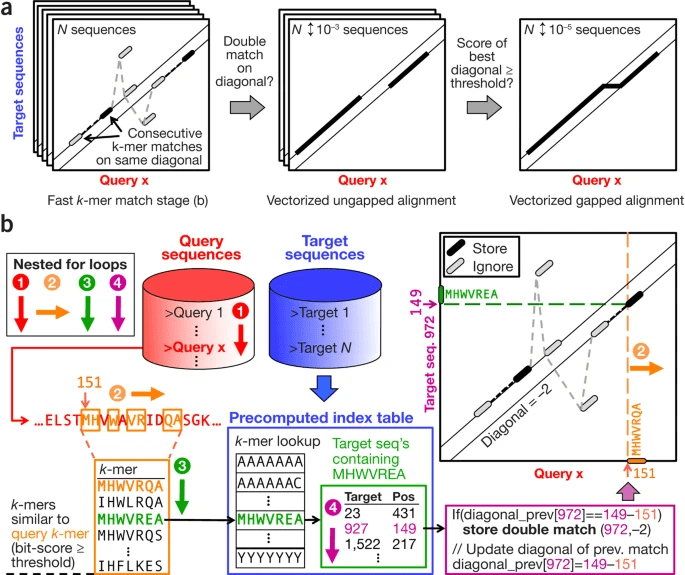
MMSeqs2 Prefilter algorithm (a lot going on in that figure, but hopefully the description helps). Source: MMSeqs2 Paper

This prefilter already cuts down the number of hits by a lot. However, the result is still to expensive for a full Smith-Waterman alignment. Part of what makes this dynamic programming algorithm very expensive is the possibility to include gaps in the alignment. Therefore, as an additional filter, the sequences that gave double diagonal hits undergo an ungapped alignment that is relatively fast (although slower than the prefilter). If the best diagonal of that alignment has a score above a predefined threshold, we finally do a proper gapped alignment and get our final result out.

mmseqs2_pipeline

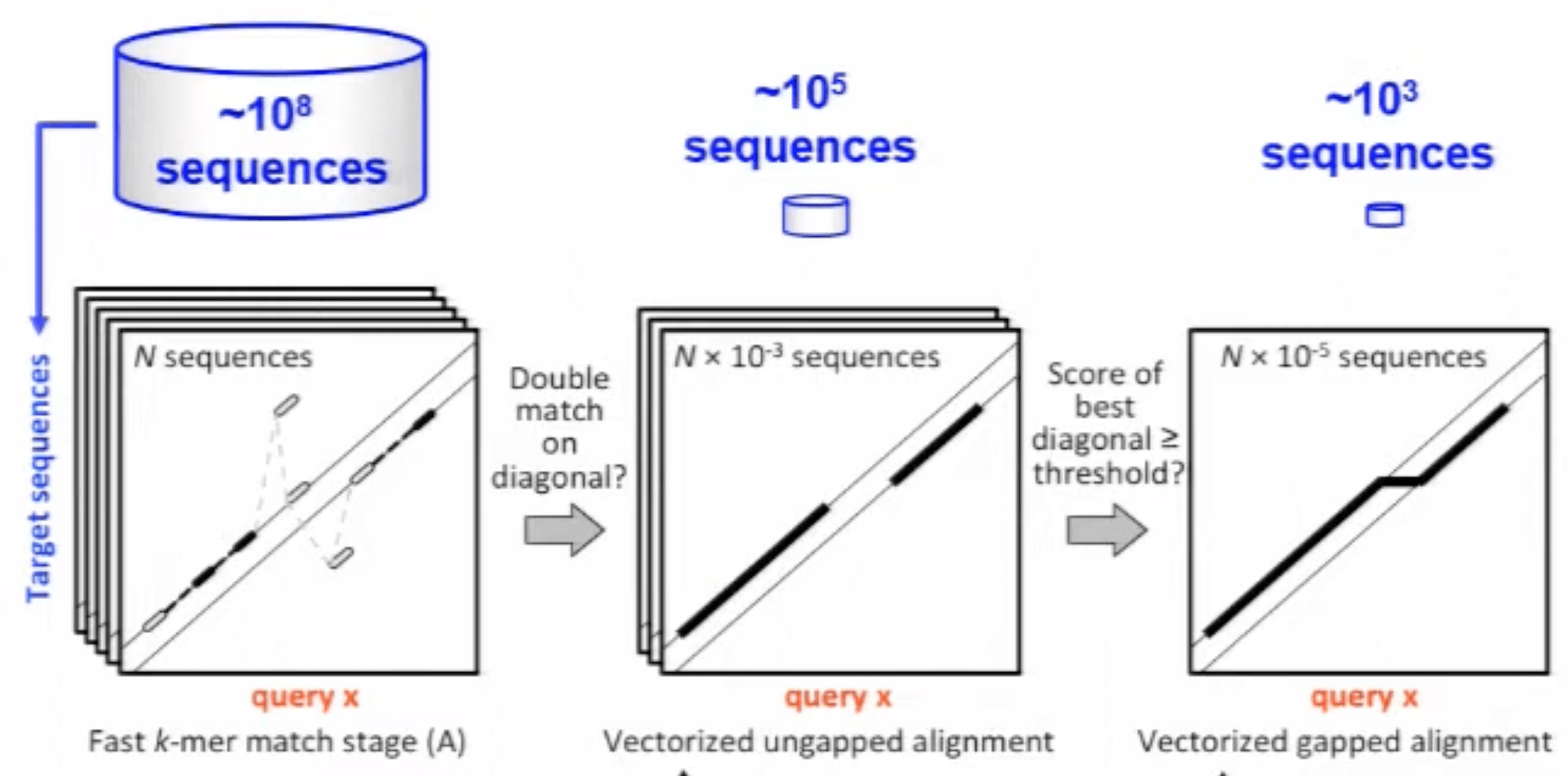
MMSeqs2 progressively filters out hits and passes them to more and more expensive alignment stages. Source: YouTube

In addition to that, the authors play all tricks in the hardware book to be fast, from AVX2 that allow 32 1-byte operations like add/mult/max to be computed in parallel per CPU clock cycle to optimising CPU cache allocation in the double diagonal hit matching stage and vectorizing both the ungapped and gapped alignment stages.

Use the prefilter for clustering

The prefiltering algorithm is not only useful for alignments, but also for sequence clustering, a task that is useful in for example creating biologically relevant train-test splits in machine learning. To cluster a sequence set with MMSeqs2, we run it either just through the prefiltering or optionally also through the alignment module and then use the output similarity graph as an input to a clustering algorithm of our choice.

If we choose the easy-cluster mode of MMSeqs2, it will just pass that similarity graph to a classic cascaded clustering algorithm. If we want to cluster large datasets, we can instead use the easy-linclust command that leverages the Linclust algorithm to cluster sequence sets in linear time, again using k-mer based analysis workflows.

Another cool property of MMSeqs2 clustering is the possibility to add new sequences to an existing clustering while maintaining stable cluster identifiers. eliminating the need to recluster the entire sequence set.

FoldSeek: structural clustering of the protein universe

Sequence alignment as described before is one of the main pillars in bioinformatics and useful for a variety of applications, from detecting homology to creating training splits for machine learning models.

However, when talking about protein structure, sequence alignments do not always tell the full story: in many cases, proteins may have very different sequences but very similar structures. This could be due to remote homology such as in the case of ubiquitin and it’s mysterious cousin Sumo which have been separated by more than 1 billion years of evolutionarity history but still are structurally strikingly similar despite a sequence identity of only 16%.

This makes the idea of structural alignment and structural clustering very appealing: with this, you could detect these remote homologies, enabling you to detect very remote homologies while also preventing your machine learning models that deal with protein structures from cheating via such examples.

However, structure alignment is quite complex: as described before, we can find an optimal solution for aligning a sequence of length $n$ to a sequence of length $m$ via dynamic programming in $O(nm)$ time since we need $n*m$ operations to populate the whole dynamic programming matrix.

For structure alignment, the problem is a lot more complicated due to the absence of natural local bounds: if we change a sequence alignment at some position, a previously aligned segment somewhere else stays unchanged. Since structural alignment operates via concerted 3D rototranslations, the introduction of gaps outside an aligned region might still affect the already aligned region due to residues that are close in 3D but far in sequence space.

Therefore, structural alignment algorithms like Dali based on distance matrices and TM-align based on the TM-score are relatively slow, preventing their application on the new scale of data we face (TM-Align would need around a year to search through the AFDB on a single CPU core). Foldseek, on the other hand, is 4-5 orders of magnitude faster and therefore suitable for such large-scale searches.

Structure to Sequence: the 3Di alphabet

How is that done? The main idea is to translate structural information into some kind of sequence-based representation that allows the use of fast sequence alignment tools. This has been tried before with tools like CLePAPS and mulPBA, but has not found widespread use due to them ony describing secondary backbone structure.These tools build on the three-letter code of helix, sheet and coil and refine it further by describing the backbone around a single residue by one of 10-20 letters. This increases the speed by reducing the problem to sequence alignment, but only captures helical and sheet-like regions well, while the large amount of information in loop regions is not captured well due to the structure there being mostly determined by interactions between different residues. In addition, neighboring residues are highly correlated (helices or sheet stretch for quite a bit in a protein), making that encoding even less informative.

FoldSeek does away with this and instead describes the tertiary instead of the backbone secondary structure via a 20-letter alphabet called 3Di. More specifically you do the following:

Select a residue to encode and its nearest 3D neighbor. They started defining “nearest” as “smallest CB-CB distance”, but then replaced that with the concept of a virtual center for reasons explained later.
Get the CA atoms of these two residues as well as the CA atoms of the residues before and after them in the sequence (in total 6), extract distance- and angle-based features from this 6-atom constellation and collect them in a 10D-descriptor.
Discretise this information into one of the 20 letters from the 3Di alphabet.

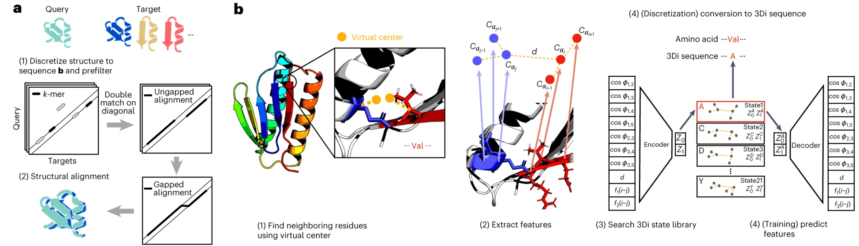
FoldSeek stages in part b of the figure. We will come back to part a. Source: FoldSeek Paper

We will talk in more detail about step 1 and 3 of this process, but you can see how the resulting 3Di sequence can be fed into any sequence-based program to get a structural alignment or clustering. In the paper, the authors show that they can do that with similar sensitivity as actual structural alignment programs, but at a fraction of the computational cost.

Virtual centers optimise conservation of interactions and tertiary vs. local interactions

The virtual center described above is determined by a pre-specified procedure described in the SI (Suppl. Fig. 1):

It lies on the plane defined by N, CA and CB
CB, CA and the virtual center form a 90 degree angle
The CA-virtual center distance is twice the CA-CB distance

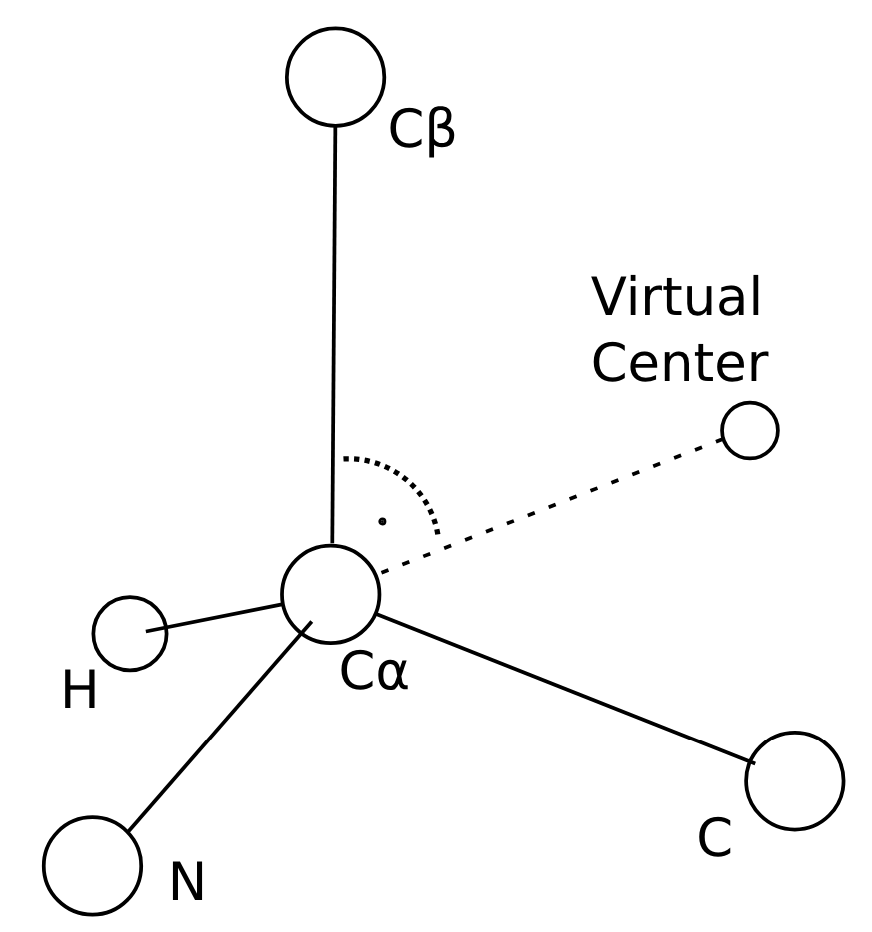
Construction of the virtual center in FoldSeek. Source: (Suppl. Fig. 1)

In the case of glycine, a virtual CB is approximated by idealising the backbone geometry as a tetrahedron.

Why is this better than just taking the CB-CB distance? Two reasons:

Conservation of Interactions: we want to make sure that in the case of structurally aligning two homologs, the nearest neighbor of residue $i$ in structure one should be the same as for residue $i$ in structure 2. If this would not be the case and we would choose a different nearest neighbor, the extracted 10D descriptor would look different, we would assign the residue different 3Di letters in the two structures and the structural alignment would fail. Empirically, they found that the CB-CB distance is not a great criterion for that and therefore came up with the virtual center definition that fulfills this desideratum more often.
Tertiary vs. local interactions: One of the downsides of the previous alphabets such as CLePAPS and mulPBA was that they have a lot of repeated information encoded by only describing local interactions as part of the secondary structure description (e.g. “these 10 residues all are in a helix”). If our 3Di alphabet ends up encoding mainly local interactions between neighbors in sequence (as would often be the case if we choose the CB-CB distance as criterion for nearest neighbor) then we end up in the same spot of mainly describing redundant local interactions. One can think about it from an information theoretic perspective in terms of mutual information: in the case of only encoding the amino acid identity, the mutual information between structurally aligned residues is the same no matter if we correct by correlation between neighbouring letters to account for local interactions or not. Other structural alphabets show a higher mutual information than pure amino acid encoding (i.e. performing only classic sequence alignment), but that difference shrinks a lot when we correct for the neighbor letter correlation. FoldSeek therefore aims to minimise the amount of local interactions it encodes and maximise the amount of tertiary interaction that is encoded. By moving the virtual center further away from the backbone and orienting it into a different direction than the CB, we achieve this goal of often encoding interactions between residues that are not neighbors in sequence.

Learning the 3Di alphabet via a VQ-VAE

Given the 10-dimensional descriptor that encodes distance- and angle-based features from the residue and its nearest neighbour as judged by the virtual center, how do we actually decide which of the 20 letters of the alphabet we assign this residue to? Well, one could do something simple like k-means clustering (which the authors started out with), but you can be smarter than that by considering the fact that our 3Di alphabet should learn maximally conserved structural states between homologs.

Therefore, the authors leverage a VQ-VAE (vector-quantized variational autoencoder) to learn the 3Di alphabet first encoding the 10D descriptor via 3-layer neural network encoder into a bottlenecked representation, than mapping it to one of the 20 discrete 3Di states (that is where the VQ part comes in) and then reconstructing the 10D descriptor again via a 3-layer neural network decoder. The crucial part here is that the reconstruction target is not the input as it is for classic VAEs. Just reconstructing the exact 10D descriptor could lead to overfitting on the exact values instead of encoding features that allow us to identify conserved states between structures. Therefore, our reconstruction target is the 10D descriptor of a structurally aligned homolog. The structural alignment in this case was part of training dataset preparation via one of the more expensive classical tools.

By targeting not the same 10D descriptor but the descriptor of a homolog, the VQ-VAE is forced to encode a discretised representation that is useful for identifying homologs, exactly the use case we are building this algorithm for. This procedure is quite clever and can be seen as similar to denoising autoencoders, where instead of swapping out the output, the input is corrupted with some noise in order for the network to learn a useful representation and avoid overfitting.

Speeding things up by building on mmseqs2

We have now trained our VQ-VAE and can use it to encode a protein structure into a 3Di sequence. We could just leave it there and leverage good-old dynamic programming via Smith-Waterman to get local alignments. But the authors were aiming for speed, so they did not stop there and took inspiration from their MMseqs2 sequence aligner described above. In fact, they use exactly the same pipeline!

In part a, we can see that Foldseek uses the same prefilter and alignment modules as MMseqs2. Source: FoldSeek Paper

Since the 3Di representation is just a sequence, we can plug that sequence into the MMseqs2 prefilter and alignment modules and get ultra-fast structural alignment. We can benefit from the clever prefilter design as well as the hardware optimisations like AVX2 instructions, optimised CPU cache, vectorisation and so on.

Applications: clustering the protein universe

Using the turbo tandem of MMSeqs2 and FoldSeek as well as integrating these advancements into structure prediction methods via ColabFold has led to a flurry of new research directions.

For one, both sequence and structure clustering is now possible on scales that were not imaginable before. The Uniclust databases was created by sequence-similarity based clustering via MMSeqs2 at 90%, 50% and 30% pairwise sequence similarity. The resulting databases showed better consistency of functional annotations than the corresponding UniRef databases, arguable due to the better clustering algorithms.

Using a combination of MMSeqs2 and Foldseek, it was possible to perform clustering on the whole AlphaFold database, identifying new putative homologs that demonstrate the value of such a resource for studying protein evolution and function on such a large scale.

Other applications opened up in phylogenetics, the study of evolutionary relationships among biological entities such as species or individuals: the use of Foldseek enabled fast homology detection via structural phylogenetics for proteins in the twilight zone, meaning that their sequence similarity is already very low but remote homology via structural similarity is still possible. In another study, a combination of MMSeqs2, ColabFold and FoldSeek enabled cross-phyla protein annotation, a task considered very challenging. Even more, protein structure prediction methods themselves were improved by applying MMSeqs2 to the Sequence Reads Archive (SRA), resulting in petabase-scale homology search and the construction of better MSAs (seems like in protein structure prediction we are now back to the old game of “who has the bigger MSA”).

While the tools as they stand right now are amazing, the algorithms behind them can still be improved. This includes making the last Smith-Waterman alignment more efficient via algorithms such as BlockAligner that uses adaptive dynamic programming with SIMD-acceleration, or even making it differentiable in order to backpropagate through the MSA construction step and enable full end-to-end-learning.

At the same time, it is still worthwile looking for other approaches to these challenges. Some of them include SWAMPNN structure alignment via ProteinMPNN that is more sensitive than FoldSeek while still being faster than many of the classical algorithms, as well as language models used to perform protein search and annotation. All in all, one can say that we can now indeed do many of the things we can do with sequences also with structures, and it will be exciting to see the scientific discoveries that result from that endeavour!

Dealing with the flood of protein structures

How protein structure prediction changed the game

FoldComp: compressing protein structures to managable sizes