The unification of representation learning and generative modelling

31 Dec 2025 in ML Last modified at: 2026-02-12

A deep dive into the convergence of discriminative and generative AI, covering 4 phases of evolution from REPA to RAE and beyond.

• Introduction
• Background
  • Generative modelling: Latent Diffusion Models
  • Representation Learning: self-supervised vision foundation models
    • From Cross-Modal Contrastive Learning to Single-Modal Contrastive Learning
    • Vision–Language Models and Sigmoid Contrastive Losses
    • Self-Distillation and Momentum Encoders
    • Masked Image Modeling and Predictive Architectures
  • Toward a Platonic Representation and Implications for Generative Models
• Overview of the Four Phases
• Phase 1: Aligning Diffusion Features to Vision Foundation Models
• Phase 2: Aligning the VAE Latent Space to Foundation Models
• Phase 3: Operating Directly in Vision Foundation Model Feature Spaces
• Phase 4: Questioning the Need for Pretrained Representations
• The Other Direction: Generative Models as Representations
  • From Pixel Prediction to Embedding Prediction
  • Diffusion Models Learn Representations Too
• Representation Learning and Alignment in Molecular Machine Learning
  • Molecular Embeddings: Borrowing from NLP and Computer Vision
  • Where to Go from Here?
• Conclusion
• Credits
• References

For the TLDR version of this post, see this version on the OPIG blog.

If you would like to cite this post in an academic context, you can use this BibTeX snippet:

@misc{didi2025r4g,
  author = {Didi, Kieran},
  title = {The unification of representation learning and generative modelling},
  url = {https://kdidi.netlify.app/blog/ml/2025-12-31-r4g/},
  year = {2025}
}

Introduction Permalink

Both generative modeling and representation learning have made impressive advances in recent years, particularly in computer vision. Diffusion ¹²³ and flow models ⁴⁵ have achieved unprecedented generation quality, while self-supervised paradigms like CLIP ⁶, DINO ⁷, and MAE ⁸ have enabled state-of-the-art performance on classification, detection, and depth estimation. Yet generation has remained separate from other vision tasks, raising a natural question: can we create unified representations useful for both discriminative and generative tasks?

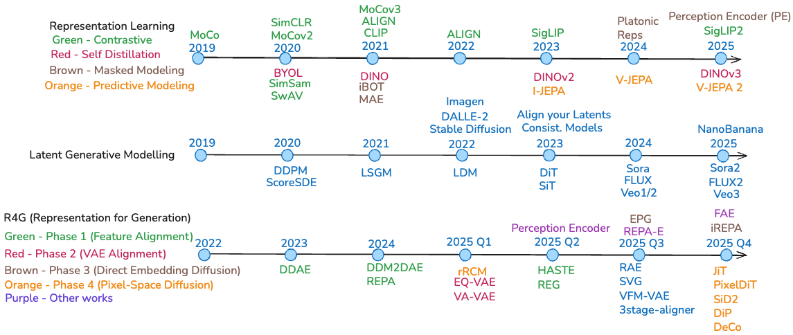Fig 1. Three parallel timelines showing the independent evolution of representation learning methods, latent generative modeling architectures, and the recent convergence of these fields in R4G (Representation for Generation).

This field—sometimes termed Representation for Generation (R4G)—has evolved rapidly over the past year, with multiple groups independently converging on similar insights. The rapid development reveals fundamental questions about visual representations: Are features learned during generation inherently different from those learned discriminatively? Can we bridge these paradigms for more efficient systems? Recent evidence suggests diffusion models already learn semantically meaningful representations ⁹¹⁰, and that generative classifiers exhibit surprisingly human-like properties ¹¹. Is there a way these two can benefit from each other more explicitly?

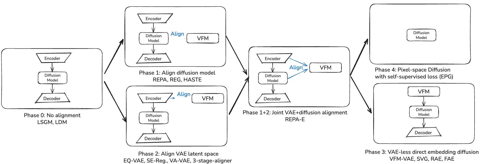Fig 2. Evolution from no alignment (Phase 0) through feature alignment (Phase 1), VAE alignment (Phase 2), and VAE-less direct embedding diffusion (Phase 3). Phase 4 (pixel-space diffusion without pretrained models) represents a parallel evolution that has been ongoing throughout, with complementary contributions to pure latent-space methods. Each block shows the architectural approach and which papers introduced key innovations.

When I started reading into the literature, I was honestly quite overwhelmed by the sheer number of papers and approaches being proposed there this year alone, with new papers coming out every week. But after some reading and discussion of some of these papers with the respective authors as well as colleagues some patterns started to emerge. In this blog post I try to organize recent developments into four phases reflecting my take on how the field developed during 2025: from initial alignment strategies to questioning whether pretrained representations are necessary at all. As part of this I also touch upon pixel-space versus latent diffusion models (again) and how the trend goes both ways, i.e. how we can use generative models for representation learning. Finally, because at heart I am a molecule guy, I share some of my thoughts on how these ideas are beginning to influence molecular machine learning, and exciting directions to pursue there.

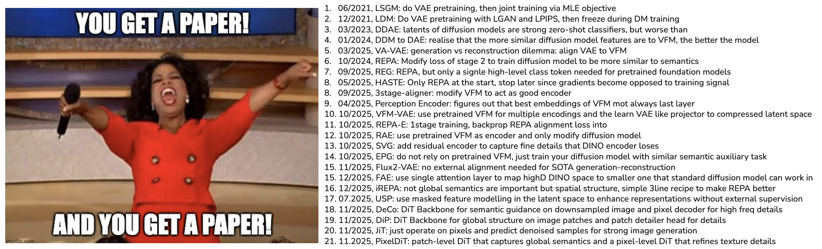Fig 3. An explosion of papers in this field has made it hard to keep an overview; by the end of this post you should hopefully be able to read any of these papers here and place it on your mental map into one of the phases we will discuss and be able to compare it to similar approaches.

Background Permalink

To talk about the unification of representation learning and generative modelling, it might be wise to shortly talk about each of these separately and review what happened in each of them recently. It has been known for quite a while that they are intimitely related (for a recent take on this see this excellent talk by Kaiming He from a CVPR2025 workshop). However, in practice they still function quite differently, both in terms of the losses and training recipes employed as well as the neural network architectures used. What is the latest in both of these fields?

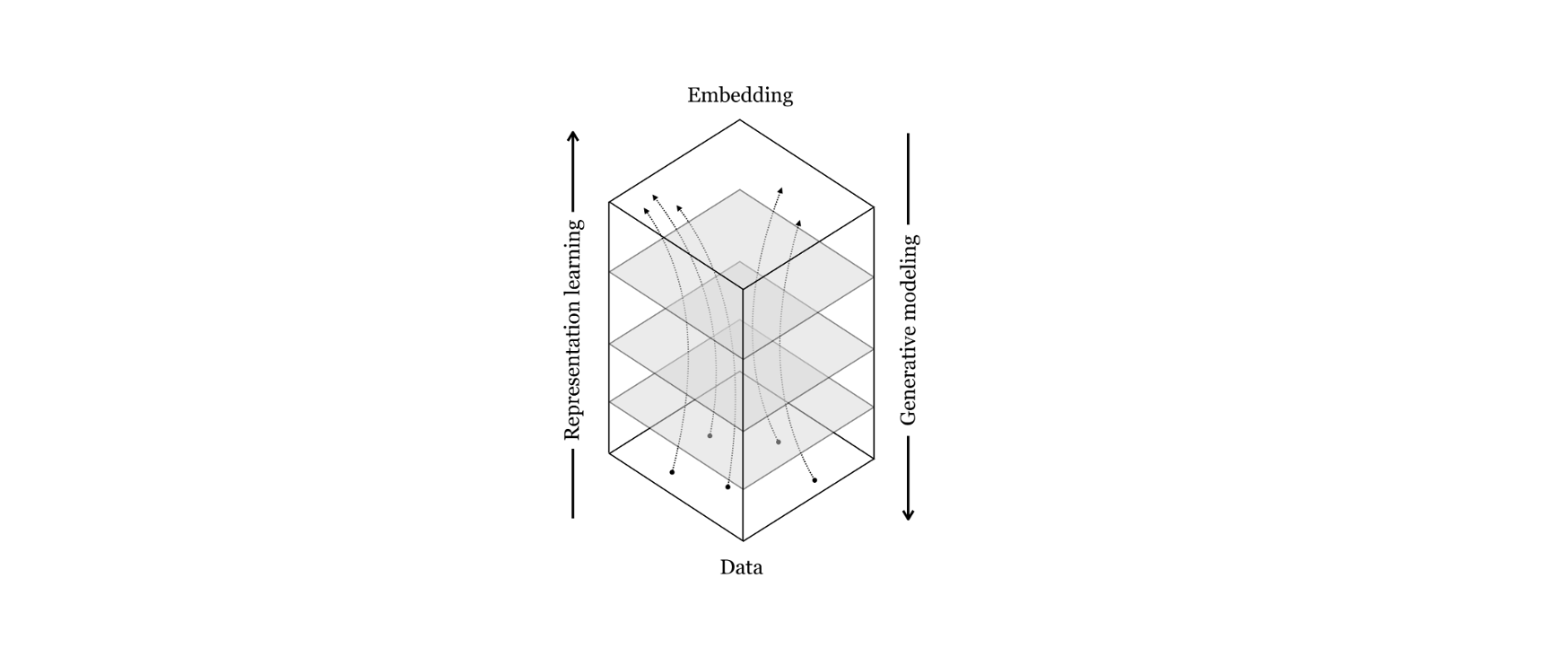
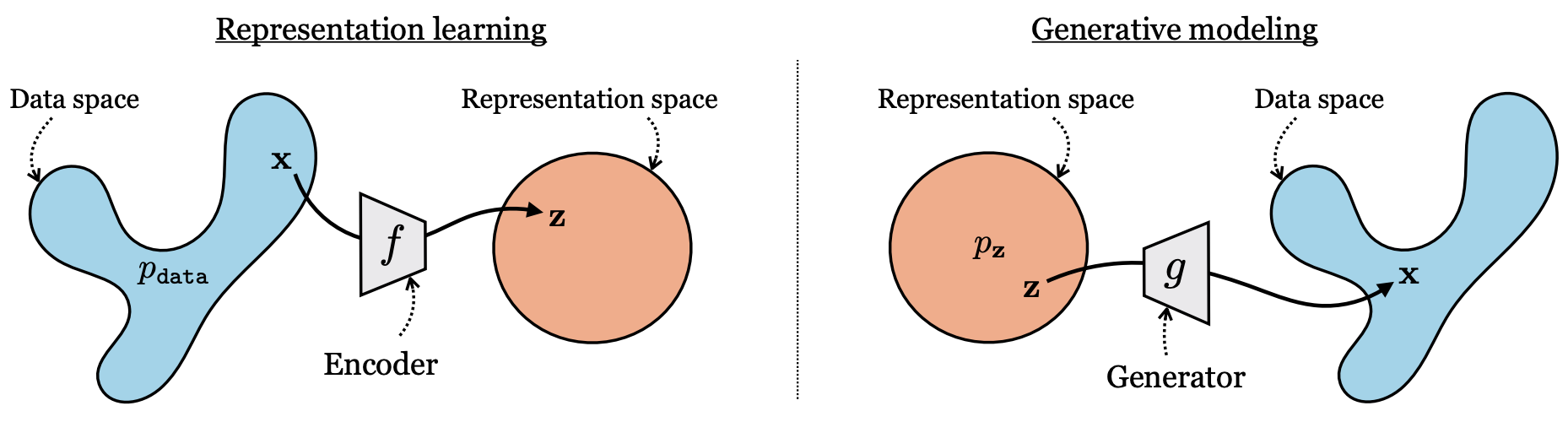Fig 4. Generative Modelling and Representation Learning are intimately connected, two sides of the same coin: while representation learning tries to map from data to some semantic representation space (e.g. to allow for easier classification of objects in an image), generative modelling wants to maps from abstract concepts like text prompts to actual data samples. Image from the “Foundation of Computer Vision” online book

Generative modelling: Latent Diffusion Models Permalink

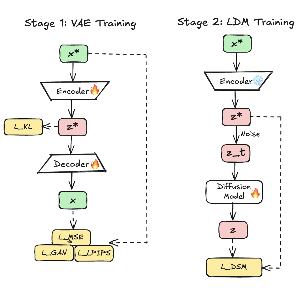Fig 5. Two-stage training: first, a VAE compresses images into latent space; second, diffusion operates in this latent space. This modular design accelerated adoption but separated tokenizer training from diffusion model training.

Diffusion models revolutionized generation by framing it as iterative denoising. While Sohl-Dickstein et al. ¹² first introduced the core idea of learning to reverse a diffusion process in 2015, the approach didn’t scale until Ho et al. ¹ introduced DDPMs that gradually add noise and learn to reverse it; Song et al. looked at it from a score-based perspective ¹³; and in 2021 they got together to formalize a unified perspective through stochastic differential equations ². This was all still in pixel-space; each pixel was denoised in RGB space, hindering both scalability as well as performance. The key breakthrough came with latent diffusion: Vahdat et al. adopted their already NVAE work ¹⁴ to propose LSGM ¹⁵, a theoretically principled framework for joint VAE+diffusion training with tractable score matching and proper variational bounds. However, despite superior theory, LSGM’s engineering complexity, including spectral regularization, careful hyperparameter tuning and variance reduction, limited practical adoption.

Rombach et al.’s Latent Diffusion Models (LDMs) ¹⁶ simplified this dramatically. Rather than joint end-to-end training, LDMs adopted a two-stage design: first, a VAE compresses images into lower-dimensional latents (typically $256 \times 256 \times 3 \to 32 \times 32 \times 4$); second, diffusion operates in this latent space. A key insight of the LDM paper—and where it fundamentally differs from LSGM—is that during autoencoding the model only encodes perceptually relevant details in the latent space, but not all fine-grained ultra high entropy information (like texture details). This pixel-level detail is re-generated in the decoder. This comes from incorporating a patch-based discriminator loss (discard local details and regenerate them) as well as the LPIPS loss (reconstruct in a feature space of perceptually relevant features) in addition to the regular MSE loss. The LDM paper calls this semantic vs. perceptual compression (see Fig. 2 in ¹⁶). This is drastically different from LSGM: in LSGM, all high-entropy local details are encoded in latent space—the same information that regular pixel-space DDPM models must model—which is why perhaps LSGM took longer to train and required bigger models in the latent space. LDM’s smart compression scheme for visual signals makes things way more scalable for image and video data. For a more in-depth discussion on latent diffusion models, see Sander Dieleman’s excellent blog ¹⁷. This simplified approach produced better perceptual quality and more stable training, allowing extension of the approach to other modalities like video generation ¹⁸¹⁹.

The modular two-stage approach provided significant advantages: VAEs pretrained once could be reused across different diffusion models, researchers could iterate independently on each component, and pretrained autoencoders from other work could be directly incorporated. This modularity accelerated research and deployment and enabled breakthroughs like Stable Diffusion XL ²⁰. However, as subsequent sections discuss, this separation between tokenizer and generative model is now being reconsidered.

Peebles and Xie’s Diffusion Transformer (DiT) ²¹ demonstrated that transformers could replace U-Nets, achieving state-of-the-art ImageNet generation with favorable scaling. DiT operates on latent patches, treating them as sequences like Vision Transformers. A key finding: model complexity correlates strongly with sample quality—increasing depth, width, or tokens consistently improves generation. The largest DiT-XL/2 model established transformers as scalable alternatives for diffusion, serving as the baseline against which subsequent alignment methods would be measured.

Recent developments have also explored alternative generative paradigms. Flow matching ⁴ provides a simulation-free approach to training continuous normalizing flows with conceptually simpler and more flexible formulations than standard diffusion. The relationship between diffusion and flow matching has been clarified ²², showing they are fundamentally equivalent under certain conditions, differing primarily in parameterization and sampling schedules—one can make a good diffusion model work just as well, and one can also define suboptimal paths in flow matching. The popularity of flow matching likely stems more from its conceptual simplicity than from clear performance advantages. These rectified flow transformers have been successfully scaled to production systems ²³.

Representation Learning: self-supervised vision foundation models Permalink

Self-supervised learning aims to learn general-purpose visual representations without manual labels, enabling models to exploit vast unlabeled corpora ^242526272829. Early approaches were largely contrastive: they defined positive and negative pairs and trained encoders so that positives map to nearby features while negatives are pushed apart ²⁴²⁵³⁰. Subsequent work progressively weakened the dependence on labels, explicit negatives, and even pixel-level reconstruction, moving toward architectures that predict high-level, semantic representations ^731322833.

From Cross-Modal Contrastive Learning to Single-Modal Contrastive Learning Permalink

A natural starting point for self-supervised representation learning is cross-modal contrastive learning, where aligned pairs provide supervision “for free.” CLIP jointly trains image and text encoders so that the similarity between matching image–caption pairs is maximized and that between mismatched pairs is minimized, using a large-scale contrastive objective over Internet-scale image-text datasets ⁶¹⁹²³. This removes the need for class labels but depends on enormous amounts of paired data, and on sufficiently many negatives in each batch to avoid trivial solutions where the model encodes only coarse semantics ³⁴.

SimCLR showed that contrastive learning can work in a purely single-modal setting ³⁰. Two heavily augmented views of the same image form a positive pair, and all other images in the batch serve as negatives. Combined with strong data augmentation, a temperature-scaled InfoNCE loss, and large encoder capacity, SimCLR achieves supervised-level performance on ImageNet, demonstrating that labels are not strictly necessary for high-quality features. However, as with most contrastive learning methods including the ones described before, this comes at the cost of extremely large batch sizes, which are needed to provide enough negative examples so that the contrastive loss encourages fine-grained, non-trivial representations rather than collapsing to coarse global features ²⁴.

SwAV improves on this regime by replacing explicit pairwise comparisons with online clustering ²⁶²⁷. Instead of contrasting features directly, SwAV assigns representations to prototype clusters and enforces consistency of these assignments across multiple augmentations of the same image. This “swapped prediction” mechanism preserves many advantages of contrastive learning while being more memory-efficient and less sensitive to batch size, making it easier to scale to large datasets and long training schedules.

Vision–Language Models and Sigmoid Contrastive Losses Permalink

Vision-language pretraining extends contrastive learning to cross-modal settings at scale. CLIP demonstrated that large-scale image-text contrastive learning yields highly transferable visual representations and strong zero-shot performance across tasks ⁶¹⁹. However, CLIP’s softmax-based loss ties batch size directly to the number of effective negatives, which complicates scaling and makes training expensive.

SigLIP addresses this by replacing the softmax contrastive loss with a pairwise sigmoid loss over image-text similarities ³⁴. This loss operates independently on each pair, enabling smaller batch sizes while still learning strong fine-grained alignments between images and text. SigLIP 2 further augments this recipe by combining contrastive training with captioning-style objectives, self-supervised losses, and improved data mixtures, leading to better semantic understanding, localization, and dense prediction performance ³⁵.

Self-Distillation and Momentum Encoders Permalink

A key limitation of contrastive methods is their reliance on negatives. BYOL and related methods showed that it is possible to dispense with explicit negatives by using a momentum-updated teacher network ³⁶³⁷. The student is trained to match the teacher’s representation of a differently augmented view of the same image; the teacher parameters are an exponential moving average of the student’s, which stabilizes training and prevents collapse in practice.

DINO extends this self-distillation paradigm and reveals several surprising properties of the resulting representations ⁷. Without labels or negatives, DINO learns features whose attention maps correspond to object boundaries and support unsupervised semantic segmentation, indicating non-trivial semantic organization. In principle, such momentum-encoder methods require only a single image per batch, since supervision comes from matching teacher and student outputs rather than contrasting with other samples.

DINOv2 scales this recipe with larger Vision Transformers, improved optimization, and a carefully curated, diverse training set ³¹. The resulting models produce highly robust and transferable features that rival or surpass supervised pretraining across many benchmarks, as well as serving as strong vision foundation encoders for downstream tasks, including generative modeling ³⁸³⁹. However, prolonged self-distillation can gradually erode fine-grained spatial information, especially in dense feature maps used for pixel-level tasks.

To address this, DINOv3 introduces Gram anchoring, a regularization that stabilizes dense feature representations over long training schedules by constraining second-order statistics across patches and scales ³². This mitigates the tendency of self-distillation to over-smooth features, preserving detailed structure that is crucial for dense prediction and generative tokenization while maintaining the semantic strengths of the DINO family.

Masked Image Modeling and Predictive Architectures Permalink

In parallel, masked image modeling treats images analogously to masked language modeling in NLP. MAE masks a large fraction of image patches (typically around 75%) and trains an asymmetric encoder-decoder architecture to reconstruct the missing pixels ⁸. This forces the encoder to focus on global structure rather than local texture, producing efficient representations that work well for many downstream tasks with modest finetuning.

iBOT combines masked prediction with self-distillation, using a teacher network as an online tokenizer that predicts semantic tokens for masked patches instead of raw pixels ⁴⁰. This hybrid objective closes much of the gap between contrastive and masked modeling approaches, yielding representations that perform strongly on both image-level classification and dense prediction.

Joint-embedding predictive architectures such as I-JEPA take a more explicitly semantic view: instead of reconstructing pixels, they predict high-level latent representations of masked regions from visible context ²⁸. By operating entirely in representation space, I-JEPA avoids over-emphasizing low-level details and focuses learning on abstract structure, leading to scalable training and strong transfer across tasks.

Toward a Platonic Representation and Implications for Generative Models Permalink

Recent work from Philip Isola’s lab at MIT has provided empirical evidence for a remarkable phenomenon: representations learned by different models, architectures, and even modalities converge toward a shared structure as models scale and training data diversifies ²⁹. This convergent behavior has motivated the Platonic Representation Hypothesis, which posits that as models grow in capacity and are trained on increasingly rich data, their internal representations converge toward a shared statistical model of reality; a “platonic” representation that is largely independent of any specific task or architecture ²⁹.

The evidence for this convergence comes from multiple angles. The foundational work demonstrates that features from independently trained vision and language models become more aligned as scale and data diversity increase, and that different self-supervised objectives yield embeddings that occupy similar subspaces up to simple linear transformations ²⁹. Subsequent research has shown that cross-modal training can benefit each modality individually: Gupta et al. demonstrate that leveraging unpaired multimodal data (e.g., text, audio, or images) consistently improves downstream performance in unimodal tasks, exploiting the assumption that different modalities are projections of a shared underlying reality ⁴¹. Perhaps most strikingly, Wang et al. show that when language models are prompted with sensory instructions (e.g., “see” or “hear”), their representations become more similar to specialist vision and audio encoders, revealing that text-only models implicitly encode multimodal structure that can be activated through appropriate prompting ⁴². This suggests that even purely text-trained language models converge toward similar representations as vision models, with the convergence becoming stronger as models scale ²⁹⁴².

This hypothesis has direct implications for generative modeling. If discriminative vision foundation models such as DINOv2, DINOv3, and MAE converge toward an approximately optimal visual representation, then explicitly leveraging these encoders can accelerate the training and improve the quality of generative models that would otherwise have to discover similar structures from scratch ^31383943. Recent work on aligning diffusion models to pretrained visual encoders—through feature alignment, representation regularization, or joint training of tokenizers and generators—can thus be viewed as an attempt to steer generative models toward this platonic representation early in training ^444546474849. This perspective sets the stage for our discussion of Phase 1 methods that explicitly align diffusion features to vision foundation models, and for later sections analyzing the emerging convergence between generative and discriminative representations.

Overview of the Four Phases Permalink

Before diving into the details, let me briefly outline the four phases and what to expect. Phase 1 introduces representation alignment—regularizing diffusion features to match pretrained vision encoders like DINOv2. Phase 2 takes this deeper by incorporating semantic structure into the VAE latent space itself. Phase 3 questions whether we need VAE compression at all, proposing to diffuse directly in pretrained representation spaces. Phase 4 represents a parallel evolution that has been ongoing throughout: improving pixel-space diffusion through architectural innovation, questioning whether pretrained representations are necessary at all.

A key insight that will emerge: spatial structure alignment matters more than global semantic information for generation quality. Methods that preserve local self-similarity patterns consistently outperform those optimizing for classification accuracy. Additionally, while these techniques are presented in the context of Latent Diffusion Models (where most scaling happens), many of the core ideas—representation alignment, semantic regularization—are general and apply equally to pixel-space methods.

It’s also worth noting that in its most general form, the “representation space” we generate from can be pure noise, as in standard pixel-space diffusion or GANs. Even in latent models, all generation ultimately originates from noise—the question is what structure we impose on the intermediate representations.

Beyond these four phases, we’ll also explore the reverse direction: how generative modeling itself can serve as a pretraining objective for learning discriminative representations. This bidirectional relationship—representations helping generation, and generation producing useful representations—suggests these paradigms may be more unified than historically assumed.

Phase 1: Aligning Diffusion Features to Vision Foundation Models Permalink

The first wave at the end of 2024/start of 2025 recognized that diffusion models learn semantically meaningful representations during training, but more slowly and less effectively than specialized discriminative models ⁵⁰⁵¹. The solution: align intermediate diffusion features with pretrained vision encoders to guide training.

REPA ⁴⁴ introduced this paradigm in October 2024 through straightforward regularization. The method extracts features from intermediate diffusion layers, projects them through small MLPs, and maximizes cosine similarity with frozen DINOv2 encoder features. This auxiliary loss complements standard denoising: $$\mathcal{L}_{\text{total}} = \mathcal{L}_{\text{diffusion}} + \lambda \mathcal{L}_{\text{align}}$$

The paper builds upon the insights from earlier work that diffusion models learn discriminative representations during denoising, but it takes the critical step to show that aligning these emerging representations with high-quality pretrained features accelerates convergence. Longer training improves weak natural alignment, but the REPA loss strengthens this alignment from the start, leading to better representations and better generation—a dual benefit suggesting a genuinely helpful inductive bias.

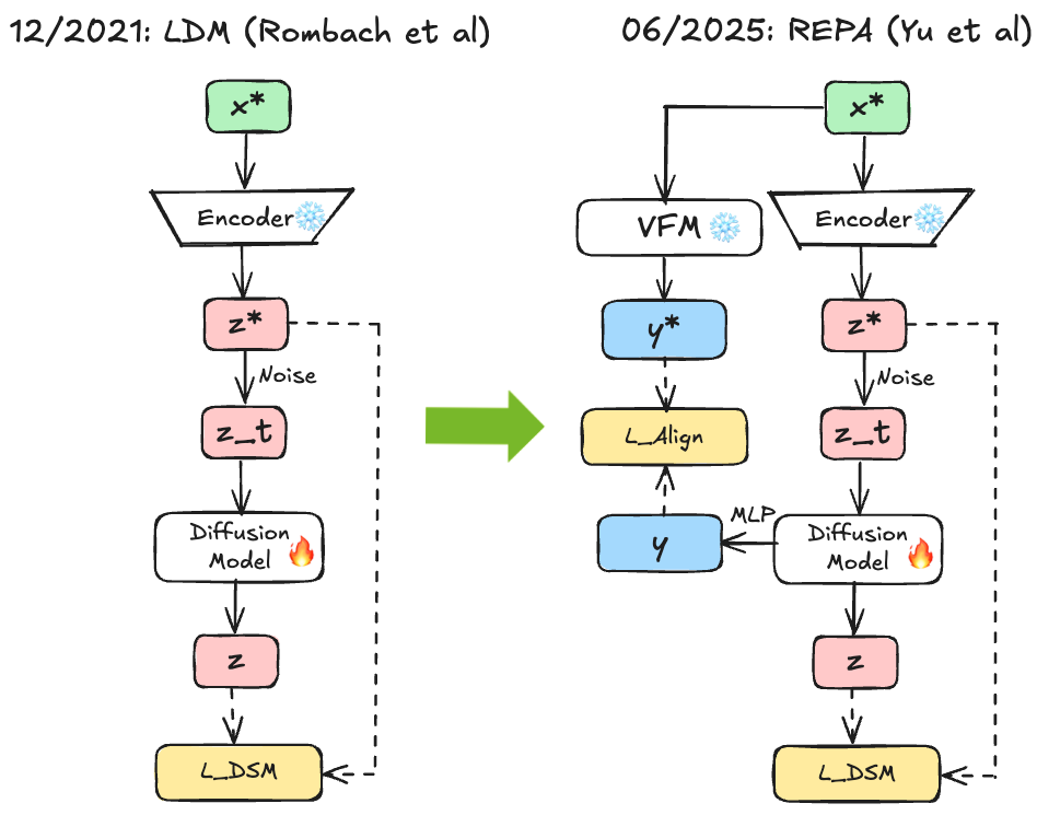Fig 6. Left shows baseline LDM architecture. Right shows REPA with alignment loss from intermediate diffusion features to frozen DINOv2 representations, speeding early training through semantic guidance.

REG ⁴⁵ extended this by entangling semantic class tokens with latent content during denoising. Rather than just aligning intermediate features, REG concatenates the [CLS] token from frozen DINOv2 with noisy latents, training the diffusion model to jointly reconstruct noise and original [CLS] token. This minimal overhead (single token, $<0.5\%$ FLOPs increase) provides stronger guidance than feature alignment alone. Interestingly, class token concatenation helps substantially even without explicit REPA alignment, though combining both works best—suggesting multiple mechanisms for incorporating semantic structure can be complementary.

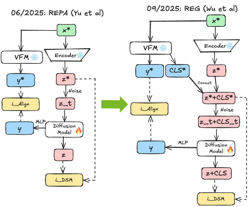Fig 7. REG concatenates the [CLS] token from frozen DINOv2 with noisy latents, enabling joint reconstruction of both image content and semantic class information directly from pure noise.

HASTE ⁴⁸ addressed a key REPA limitation: alignment helps dramatically early but can plateau or degrade later. Once the generative model begins modeling the full data distribution, the lower-dimensional discriminative teacher becomes a constraint rather than guide. The discriminative encoder focuses on task-relevant semantics while discarding generative details; forcing continued alignment may prevent learning the distribution’s full complexity. HASTE introduces two-phase training: Phase I simultaneously distills attention maps (relational priors) and feature projections like REPA (semantic anchors) for rapid initial convergence. Phase II terminates alignment at a predetermined iteration, freeing the model to exploit its generative capacity. This simple modification achieves dramatic acceleration, with the key insight that alignment is most valuable for initial structure but counterproductive once basic semantic organization is learned.

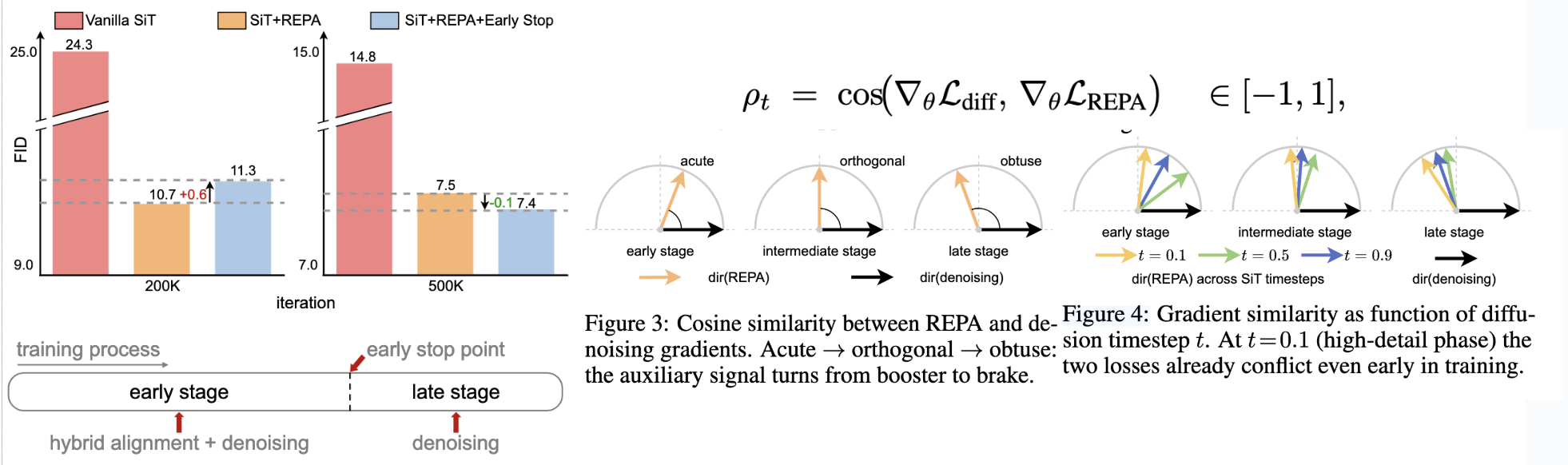Fig 8. Phase I applies holistic alignment distilling both attention maps and features. Phase II terminates alignment one-shot at a fixed iteration, freeing the diffusion model to model the full distribution without the discriminative teacher constraint.

Several puzzling trends emerged in representation alignment that defied conventional understanding. Larger model variants within the same encoder family often led to similar or even worse generation performance despite higher ImageNet-1K accuracy—DINOv2’s larger variants showed diminishing returns, while PE and C-RADIO exhibited this counterintuitive pattern even more starkly⁴⁴. More strikingly, representations with dramatically higher global semantic understanding consistently underperformed: PE-Core-G (82.8% ImageNet accuracy) generated worse images than PE-Spatial-B (53.1% accuracy), and SAM2-S achieved strong generation performance despite only 24.1% ImageNet accuracy - approximately 60% lower than many competing encoders. Perhaps most revealing, controlled experiments showed that explicitly injecting global information through CLS token mixing improved linear probing accuracy from 70.7% to 78.5% while simultaneously degrading generation quality, with FID worsening from 19.2 to 25.4.

iREPA’s analysis in December 2025⁵² resolved these contradictions by demonstrating that spatial structure—the self-similarity patterns between patch tokens—not global semantics, drives representation alignment effectiveness. To quantify this insight, the authors measured spatial self-similarity structure ⁵³ across patch tokens and performed large-scale correlation analysis across 27 vision encoders and three model sizes. Spatial structure metrics exhibited remarkably strong correlation with generation FID (Pearson |r| > 0.852 for metrics like Local Distance Similarity, Short-Range Spatial Similarity, Cosine Distance Similarity, and Relative Mean Spatial Contrast), far exceeding ImageNet-1K accuracy’s predictive power (|r| = 0.26). ​ This explained SAM2’s paradoxical success: despite poor classification accuracy, it maintained strong spatial structure that proved ideal for generation. The authors then took this further and made two small modifications to the REPA recipe: by replacing standard MLP projection with convolutional layers that preserve local spatial relationships and implementing spatial normalization to accentuate relational structure transfer, iREPA (implemented in fewer than 4 lines of code) consistently improves convergence speed across diverse encoders, model sizes, and training recipes including REPA, REPA-E (more on this later), and MeanFlow (a few-step training method). This aligns with HASTE’s emphasis on attention distillation: the success lies in teaching spatial organization coherence rather than transferring high-level semantic concepts.

These findings are quite intuitive when you think about what generative models need to do: they must model all spatial structure in detail, which is expensive to discover from scratch. In contrast, global semantic understanding is more relevant for classification than for pixel-level generation. A model that knows “this is a dog” but doesn’t understand the spatial relationships between patches will generate poorly, while a model with strong spatial coherence but weaker global semantics can still produce coherent images.

Another angle to think about why alignment helps is that the diffusion training objective is inherently high variance: at each iteration, we present a noisy input $\mathbf{x}_t$ and ask the model to predict $\mathbf{x}_0$, but the optimal prediction is not any single $\mathbf{x}_0$ seen during training—it’s the expectation $\mathbb{E}[\mathbf{x}_0 \mid \mathbf{x}_t]$ over all possible clean images consistent with that noisy input ⁵⁴. At high noise levels, this expectation corresponds roughly to the mean of the entire dataset. The model must learn to implicitly average over many possible reconstructions, but it only ever sees individual samples as supervision. This mismatch between what we supervise (samples) and what we want (expectations) makes the objective noisy and slows representation learning.

Representation alignment methods like REPA address this by providing a low-variance auxiliary signal. The pretrained vision encoder already captures useful spatial and semantic structure through objectives that don’t suffer from this sample-vs-expectation mismatch. By aligning to these representations, we essentially provide the denoiser with a shortcut to the internal structure it needs for effective denoising, bypassing the slow process of discovering this structure through the high-variance diffusion objective alone.

In summary, phase 1 establishes clear patterns: Using pretrained vision foundation models through representation alignment dramatically accelerates diffusion training. However, the methods operate at the level of intermediate diffusion features, leaving the VAE latent space unchanged. Phase 2 takes the logical next step: incorporating semantic structure into the latent space itself.

Phase 2: Aligning the VAE Latent Space to Foundation Models Permalink

While Phase 1 aligned intermediate diffusion features, Phase 2 recognized that the latent space itself—the compressed VAE representation—could incorporate semantic structure from vision foundation models. This deeper integration addresses the fundamental trade-off between reconstruction quality and learnability of the latent distribution.

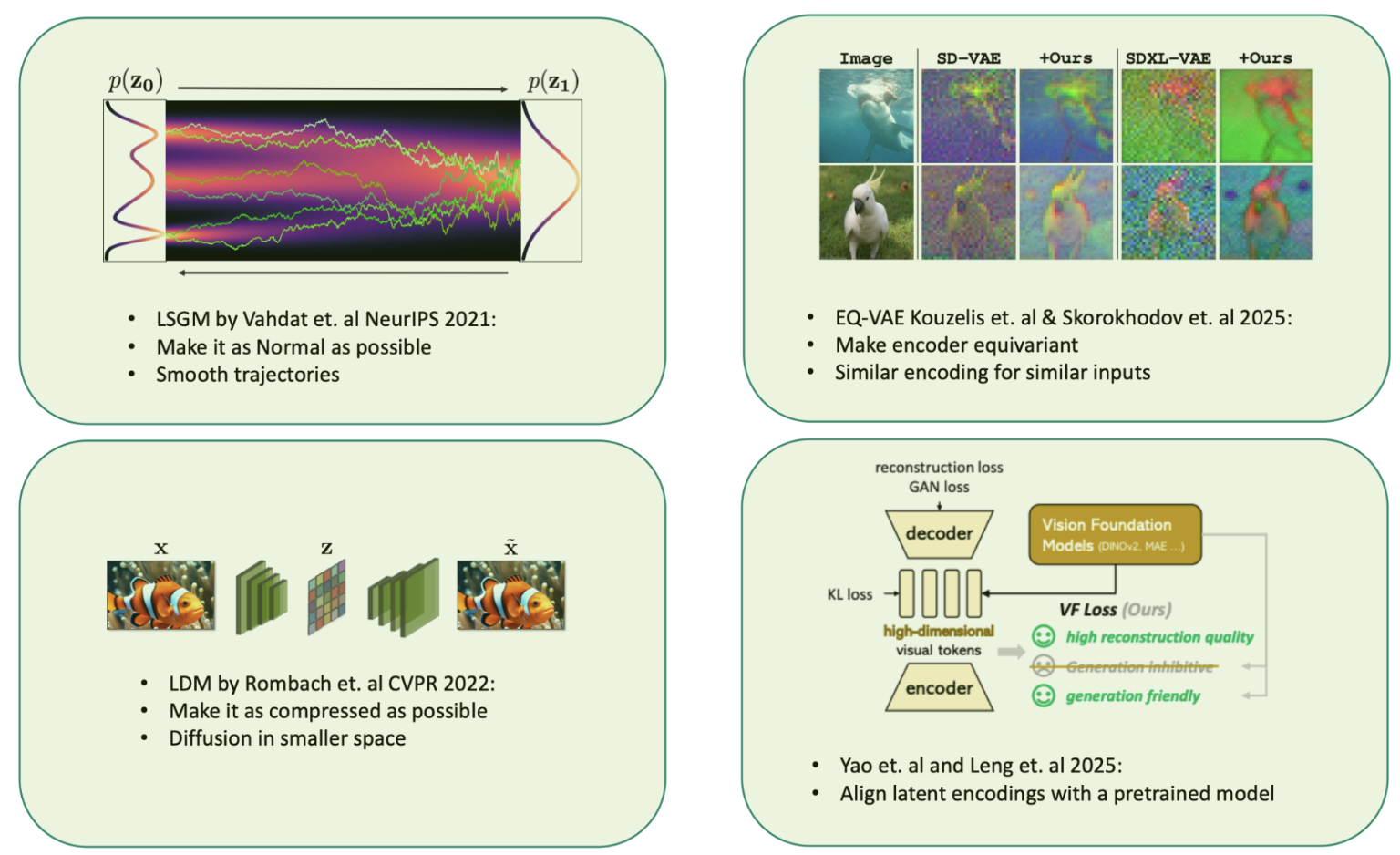Fig 9. LSGM (2021) aims for smooth trajectories in latent space by normalizing distributions. LDM (2022) emphasizes highly compressed latents for computational efficiency. EQ-VAE and VA-VAE tackle the trade-off: improving encoder equivariance and aligning latent encodings with pretrained models to create learnable high-dimensional spaces. Image kindly adapted from Arash Vahdat.

Standard LDM treats VAE and diffusion training as independent, with the VAE optimized solely for pixel reconstruction (and perceptual quality by auxiliary losses relying on discriminators or metrics like LPIPS ¹⁷). This pixel-focused objective produces latents encoding low-level details effectively but lacking semantic structure. Increasing latent dimensionality improves reconstruction but creates higher-dimensional, more complex spaces for diffusion to learn—an “optimization dilemma” where better reconstruction leads to harder generation.

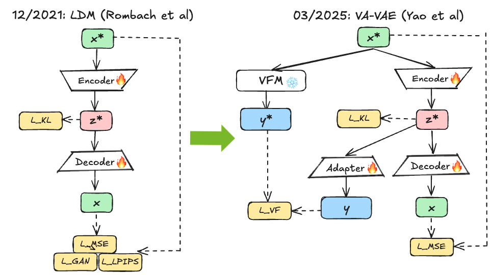Fig 10. VAE encoder trains with both reconstruction loss and alignment loss to frozen VFM features, creating latents that are both reconstructive and semantically meaningful for efficient diffusion model training.

VA-VAE ⁴⁷ directly tackles this: it aligns the VAE’s latent space with pretrained vision foundation models during tokenizer training rather than relying solely on pixels via their VF loss: $$\mathcal{L}_{\text{VA-VAE}} = \mathcal{L}_{\text{recon}} + \beta \cdot \text{KL} + \lambda_{\text{align}} \mathcal{L}_{\text{VF}}.$$ $$\mathcal{L}_{\text{VF}} = w_{\text{hyper}} \, w_{\text{adaptive}} \Big( \mathcal{L}_{\text{mcos}} + \mathcal{L}_{\text{mdms}} \Big).$$

with $$\mathcal{L}_{\text{mcos}} = \frac{1}{h w} \sum_{i=1}^{h} \sum_{j=1}^{w} \operatorname{ReLU} \!\left( 1 - m_{1} - \frac{z'_{ij} \cdot f_{ij}} {\lVert z'_{ij}\rVert \,\lVert f_{ij}\rVert} \right),$$ $$\mathcal{L}_{\text{mdms}} = \frac{1}{N^{2}} \sum_{i,j} \operatorname{ReLU} \left( \left| \frac{z_i \cdot z_j}{\lVert z_i\rVert \,\lVert z_j\rVert} - \frac{f_i \cdot f_j}{\lVert f_i\rVert \,\lVert f_j\rVert} \right| - m_{2} \right),$$

where $z$ denotes latent vectors from the VAE latent feature map and $f$ denotes vectors from the frozen vision foundation feature map for the same image; $Z' = WZ$ linearly projects VAE latents to the VFM feature dimension; $z'_{ij}$ and $f_{ij}$ are the projected latent and VFM feature at spatial position $(i,j)$; $z_i, f_i$ are vectors at position $i$ after flattening the $h \times w$ grid into $N = h w$ tokens; $m_1$ and $m_2$ are cosine-similarity margins; $\mathcal{L}_{\text{mcos}}$ enforces pointwise alignment, $\mathcal{L}_{\text{mdms}}$ aligns pairwise relational structure; $w_{\text{adaptive}} = \lVert\nabla \mathcal{L}_{\text{recon}}\rVert / \lVert\nabla \mathcal{L}_{\text{VF,raw}}\rVert$ rescales VF gradients to match the reconstruction loss, and $w_{\text{hyper}}$ is a user-set scalar (e.g., $0.1$) controlling the overall VF strength.

The VF loss encourages both point-by-point alignment (individual latent vectors close to VFM features) and relative alignment (relationships between latents match relationships between features), using adaptive weighting similar in spirit to loss balancing in GANs ⁵⁵. This yields semantically organized high-dimensional latent spaces that retain reconstruction quality while being more learnable for downstream generative models.

By semantically structuring the latent space of the VAE, it reduces the diffusion model’s burden, allowing it to focus on learning the distribution rather than also discovering semantic organization. The latent space provides appropriate inductive bias—semantic structure “baked in” through VFM alignment while pixel details are captured through reconstruction.

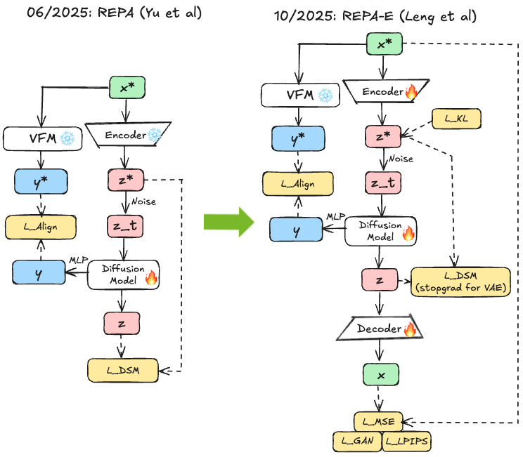
Fig 11. Left shows stage-wise training with frozen VAE. Right shows REPA-E with careful gradient flow: alignment loss flows to both components, diffusion loss uses stop-gradient on VAE encoder, and VAE receives alignment gradients through BatchNorm for latent normalization.

After diffusion model alignment as well as VAE alignment had been demonstrated, REPA-E ⁴⁶ takes integration further through joint VAE+diffusion training, challenging the convention that these components should train separately. It demonstrates that while naive end-to-end training with diffusion loss alone is ineffective (causing latent space collapse), representation alignment provides necessary constraints for successful joint optimization. The key innovation proved to be careful gradient control. Alignment loss flows to both VAE and diffusion model, but diffusion loss uses stop-gradient on the VAE encoder to prevent collapse (the VAE shouldn’t change to make diffusion easier at reconstruction’s cost). In addition, to keep the latent space normalised, the VAE receives alignment gradients only through BatchNorm normalisation. This enables joint optimization: the VAE improves to produce latents both reconstructive and well-aligned, while the diffusion model learns in this evolving but stable space. Joint optimization improves the VAE itself, leading to better latent structure (higher VFM alignment, better class separation) and downstream performance. While in LSGM ¹⁵ pretraining of the VAE was necessary, true end-to-end training is now possible.

3-Stage-Aligner ⁵⁶ proposes an alternative strategy: rather than training the VAE from scratch with alignment, freeze a pretrained encoder (e.g., DINOv2), map into into a low-dimension space via an adapter block and learn to align a decoder through three stages. Stage 1 (Latent Alignment) freezes the VFM encoder and trains the adapter plus decoder, establishing a semantic latent space with basic reconstruction capabilities. The resulting latents are semantically grounded but exhibit color shifts and missing fine-grained details since the frozen encoder was not trained for reconstruction. Stage 2 (Perceptual Alignment) jointly optimizes adapter and encoder (now unfrozen) with semantic preservation loss maintaining alignment with original frozen VFM features: $$\mathcal{L}_{\text{Stage 2}} = \mathcal{L}_{\text{recon}} + \lambda_2 \lVert\text{Enc}(x) - \text{Enc}_{\text{frozen}}(x) \rVert^2$$

The L2 loss prevents encoder drift from the pretrained semantic structure while allowing capture of fine-grained color and texture. Stage 3 (Decoder Refinement) freezes both encoder and adapter, allowing the decoder to better exploit the latent representation changed during Stage 2 without disturbing semantic structure.

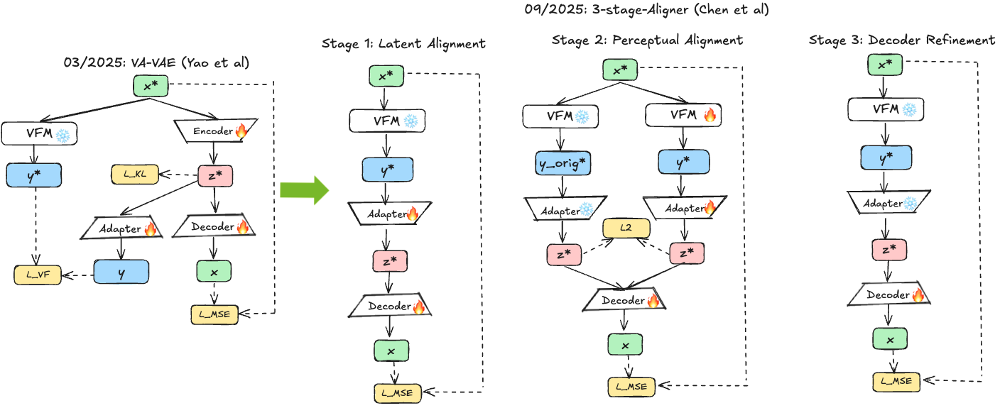Fig 12. Stage 1 establishes semantic grounding with frozen encoder. Stage 2 allows encoder refinement with semantic preservation loss. Stage 3 optimizes decoder for reconstruction quality, carefully balancing semantic preservation with fine-grained detail capture.

This yields semantically rich tokenizers where latent space inherits discriminative structure from the pretrained encoder. The three-stage process carefully balances semantic preservation (maintaining VFM structure) with reconstruction quality (capturing fine-grained details), avoiding color shifts of purely frozen encoders and semantic drift of fully unconstrained fine-tuning. Note the contrast with REPA-E’s end-to-end approach: 3-Stage-Aligner returns to explicit staged training rather than joint optimization. This reflects a broader pattern in Phase 2—there’s a zoo of different methods (end-to-end vs. staged, joint vs. separate alignment) and it remains unclear which approach is definitively best, as many of these concurrent works don’t directly compare to each other under identical conditions.

Phase 2 establishes that incorporating semantic structure directly into VAE latent space—whether through alignment loss during training (VA-VAE), end-to-end joint optimization (REPA-E), or staged adaptation of frozen encoders (3stage-aligner)—produces superior results compared to standard pixel-focused VAE training. These semantically-structured spaces are easier to learn (faster convergence) and produce better final quality. However, they still rely on the two-stage VAE+diffusion pipeline, raising a natural question: do we need VAE compression at all?

Phase 3: Operating Directly in Vision Foundation Model Feature Spaces Permalink

The third phase represents a more radical departure, questioning whether the VAE bottleneck is necessary at all. Instead of compressing images through a VAE and then aligning the latent space, these methods propose directly using pretrained vision foundation model features as the “latent space” for diffusion, or training autoencoders specifically to preserve discriminative information rather than minimize reconstruction error.

Based on the observation made in Perception Encoder ⁵⁷ that the best visual embeddings for downstream tasks are often not at the output of vision networks but rather in intermediate layers, VFM-VAE ⁴³ merges frozen VFM features from different parts of the network as latent representations. However, VFMs focus on semantic understanding, producing spatially coarse features (e.g., DINOv2 ViT-L outputs $16 \times 16$ for $256 \times 256$ images) sacrificing pixel fidelity. VFM-VAE redesigns the decoder with multi-scale latent fusion (combining features from multiple VFM layers, providing both semantic guidance from deep layers and spatial detail from shallow layers) and progressive resolution reconstruction (building up resolution gradually through decoder blocks, starting from coarse VFM features and progressively adding detail). In addition, the embedding dimensionality of VFMs is often too high for effective generative modelling; VFM-VAE circumvents this by mapping the different embeddings into a compressed latent space that is regularised via KL divergence, thereby still containing a VAE but with strong initialisation by a VFM.

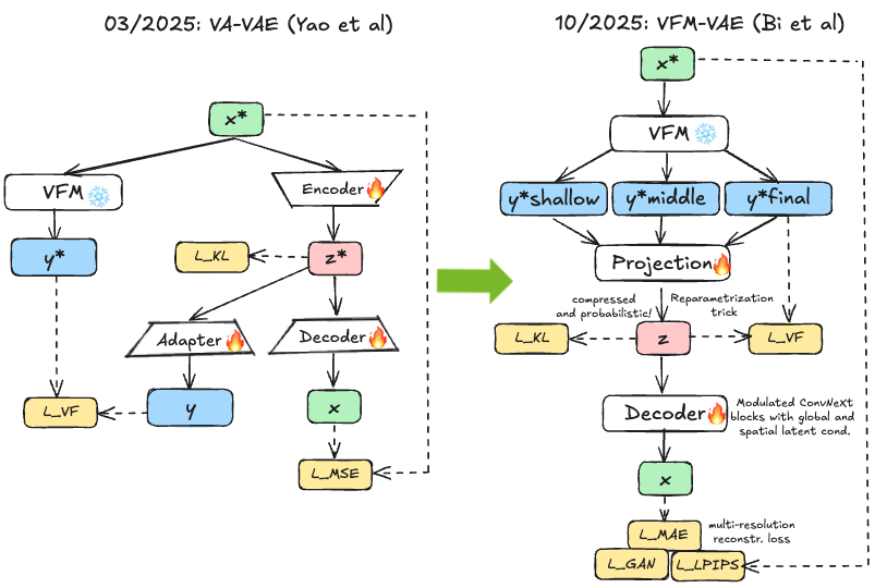
Fig 13. In VFM-VAE, multiple VFM encodings are compressed into a single latent representation that is then projected out to pixel space via multi-scale decoders. The right side shows that this latent space is more robust to geometric perturbations and achieves strong reconstruction as well as generation.

This enables high-quality reconstruction from semantically rich but spatially compact representations. The work also introduces SE-CKNNA metric for diagnosing representation dynamics during diffusion training. SE-CKNNA measures how well semantic structure in latent space is preserved during noising, revealing that semantic structure degrades nonlinearly with noise level, with critical thresholds where class separability breaks down. Using these insights, the authors develop joint tokenizer-diffusion alignment strategy dramatically accelerating convergence. The frozen pretrained encoder ensures the latent space maintains semantic alignment even under distribution shifts—Phase 2 methods that fine-tune encoders risk semantic drift; VFM-VAE’s frozen encoder ensures consistent structure. However, this requires architectural innovations (multi-scale fusion, progressive reconstruction) to overcome reconstruction challenges of coarse frozen features, which prevents easy adoption.

SVG ⁵⁸ tries to avoid these complex architectural modifications by taking a principled approach analyzing why VAE latent spaces are problematic: they lack clear semantic separation and strong discriminative structure. Standard VAE latents exhibit semantic entanglement (different classes overlap) and poor class compactness (same-class samples widely dispersed). This makes the distribution difficult for diffusion to learn, as it must simultaneously discover semantic structure and model fine-grained variation. To overcome this, SVG constructs latent representations from frozen DINO features providing semantically discriminative structure with clear class separation, augmented with lightweight residual branch capturing fine-grained details: $$z_{\text{final}} = z_{\text{DINO}} + \alpha \cdot z_{\text{residual}}$$

where frozen DINOv2 provides semantics and a learned residual encoder captures color, texture, and other details DINO discards. Normal VAE latents are semantically entangled, but alignment to VFM models enables clearer class separation and more compact classes. The SVG encoder proves important for fine-grained color details. No diffusion model tricks are needed since in the case of the chosen VFM DINOv3, the latent space is small enough (384-dimensional) to be modelled without compression. However, the alignment loss is crucial: without it, the decoder over-relies on the residual encoder, and numerical range differences between normalized frozen DINOv3 features and unnormalized learned residuals can distort semantic embeddings.

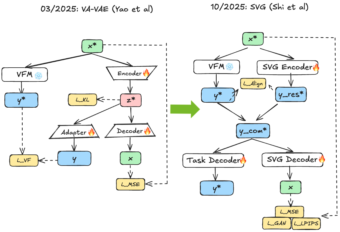Fig 14. Left shows VA-VAE with learned encoder aligned to VFM. Right shows SVG with frozen DINO encoder plus lightweight residual encoder capturing fine-grained details, enabling clearer semantic separation without VAE training.

While SVG emphasises the need for a modest embedding space dimensionality and the need for a residual encoder that makes up for missing pixel-level details in the VFM embeddings, RAE ⁵⁹ tries to replace the VAE solely with pretrained representation encoders paired with trained decoders, without additional compression or auxiliary encoders. The authors systematically explore encoders from diverse self-supervised methods (DINO, SigLIP, MAE) and analyze challenges of operating diffusion transformers in resulting high-dimensional spaces. While standard VAE latents are low-dimensional ($32 \times 32 \times 4$, or 4K dimensions), representation encoder outputs are much higher ($16 \times 16 \times 1024$ for DINOv2 ViT-L, or 262K dimensions). This poses challenges for diffusion transformers that generally perform poorly in such high-dimensional spaces.

RAE identifies and addresses sources of difficulty through theoretically motivated solutions. First, standard DiT bottlenecks all tokens through the same hidden dimension, so when input tokens have higher dimensionality, this creates an information bottleneck. RAE introduces a wide DDT head that maintains high-dimensional representations through a final shallow-but-wide layer while keeping the majority of the DiT block lower-dimensional. Second, standard schedules are designed based on spatial dimensions assuming certain statistical properties. Representation encoder outputs have different characteristics (already normalized, different variance structure). Therefore, RAE makes the noise schedule depend on actual data statistics rather than assuming fixed properties. Third, since the decoder trains separately from the frozen encoder, mismatch can occur at inference—the diffusion model produces slightly imperfect samples, but the decoder was trained on clean representations. Following TarFlow ⁶⁰, RAE adds noise augmentation during decoder training for robustness to imperfect samples.

RAE demonstrated that high-quality reconstruction from frozen DINO encoders with strong representations is possible. Computational overhead is minimal since DiT cost depends mostly on sequence length, not token dimension (which the wide head addresses). The DiT adjustments are necessary: scaling width to token dimension, making noise schedule data-dependent instead of spatial-dependent, and using noise-augmented decoding due to discrete decoder training. An additional benefit of RAE is that high-resolution synthesis is trivially enabled by swapping decoders with different patch sizes—the frozen encoder and trained diffusion model remain unchanged.

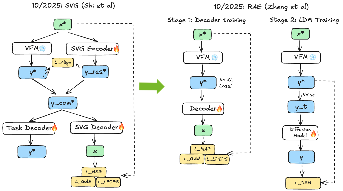Fig 15. Shows systematic exploration of different pretrained encoders (DINO, SigLIP, MAE) as frozen latent encoders, with DiT adjustments (wide DDT head, data-dependent noise schedule, noise-augmented decoding) enabling effective diffusion in high-dimensional representation spaces.

However, while RAE allowed the direct use of pretrained VFMs as encoders, it has two main limitations:

1. The modifications of the diffusion model required to make this work were substantial.
2. There is no emphasis whatsoever on reconstruction, limiting editing capabilities of these models and making them potentially vulnerable to drifting off the data manifold.

FAE ⁶¹ focuses on tackling the first of these challenges by introducing a simple adoption via a single attention layer that allows the usage of standard LightningDiT recipes. By then training to both reconstruct images and preserve pretrained features, FAE creates truly unified representation serving as both generative latent space and discriminative feature space. The simple translation layer (a single attention layer between frozen encoder features and generative decoder) provides minimal but effective transformation. This allows use of standard diffusion models again without the RAE modifications, demonstrating that the right architectural intervention can eliminate the need for extensive model adjustments. It also shows that the simple translation layer preserves the spatial structure in latent space, which aligns with the iREPA insights that spatial structure is the main determinant for how effective alignment will be for generation quality ⁵². While these tricks seem useful to avoid the RAE architecture modifications like noise-augmented decoding and wide DDT head, recent work suggests that these modifications are not necessary once one scales RAE models up to larger sizes where the DiT width is anyway larger than the VFM embedding space ⁶².

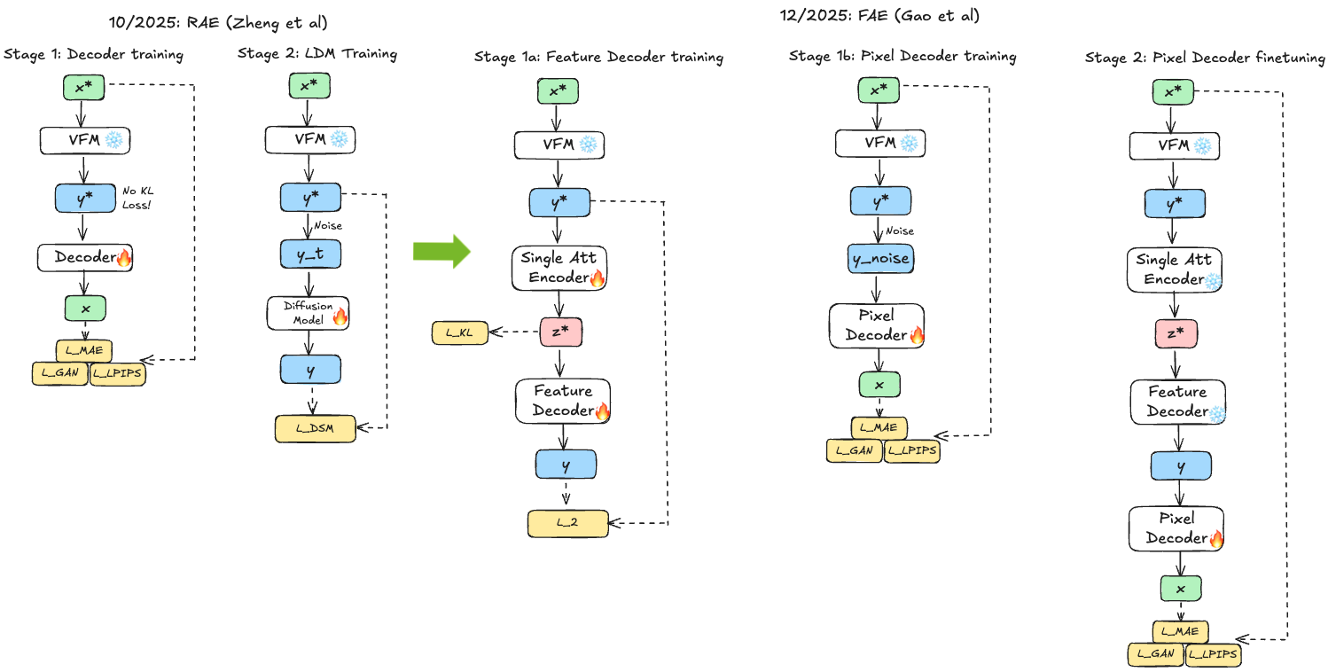Fig 16. Unlike RAE, FAE introduces a lightweight “translation layer” (a single attention block) to align frozen pretrained encoder features with the generative decoder. This minimal intervention preserves spatial structure and discriminative power.

An alternative perspective on RAE’s convergence difficulties argues that the problem is fundamentally geometric, not architectural. Standard flow matching uses linear interpolation between noise and data, creating probability paths that cut through Euclidean space. When data lies on a curved manifold—such as the hypersphere that representation encoders like DINOv2 produce—these straight-line paths pass through low-density regions in the interior of the manifold rather than following its surface. This “Geometric Interference” causes standard diffusion transformers to fail on representation spaces.

RJF (Riemannian Flow Matching with Jacobi Regularization) ⁶³ addresses this by explicitly modifying the probability paths: when the manifold geometry is known (a hypersphere for DINO features), it replaces linear interpolation with geodesic interpolation (SLERP), constraining paths to follow the manifold surface using Riemannian flow matching ⁶⁴. It additionally corrects for curvature-induced error propagation via Jacobi regularization ⁶⁵. This enables standard DiT architectures to converge without width scaling: a DiT-B (131M parameters) achieves FID 3.37 where prior methods fail entirely. RJF is in spirit similar to CDC-FM (Carré du champ flow matching) ⁶⁶, which also modifies probability paths to respect data geometry; the key difference is that RJF requires explicit knowledge of the manifold (enabling geodesic paths), while CDC-FM estimates local curvature from data via geometry-aware noise covariances, making it more general but less precise when the manifold structure is known.

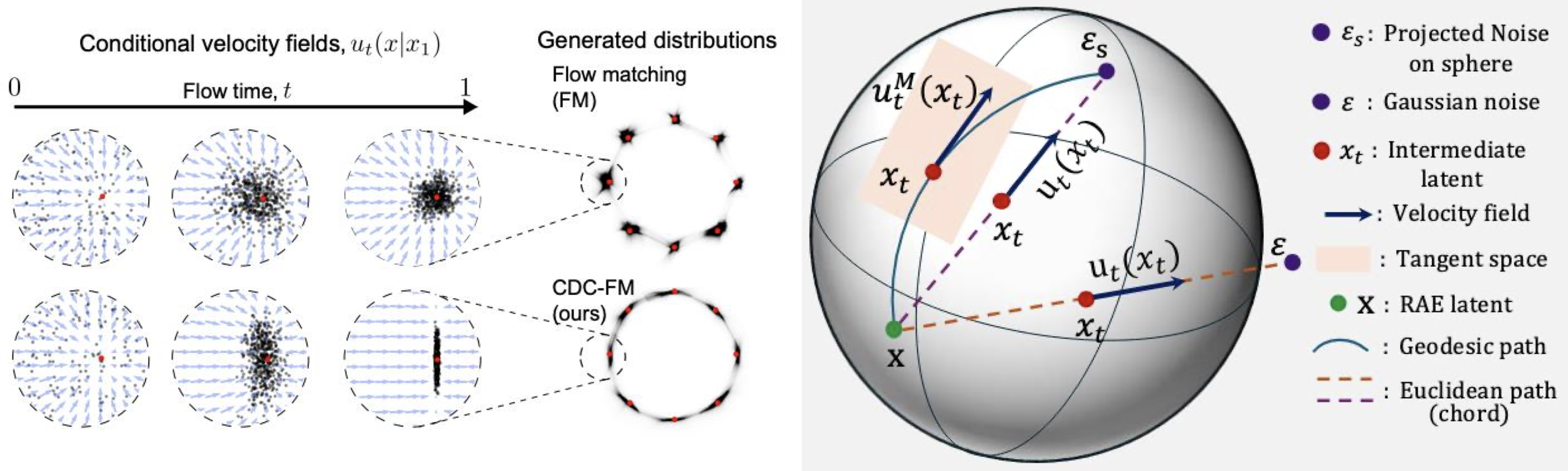Fig 17. Both CDC-FM (left) and RJF (right) modify the probability path structure to follow the data manifold structure, with CDC-FM using a spatially varying, anisotropic Gaussian noise whose covariance captures local manifold geometry and RJF using Riemannian flow matching and Jacobi regularization.

While FAE and RJF tackled the architectural adoption problem of RAE, PS-VAE ⁶⁷ tackled the editing problem that comes with the fact that RAE does not encourage the latent space to encode reconstruction capability explicitly. By training sequential representation as well as pixel decoders as well as finetuning the pretrained representation encoder with reconstruction losses, they find a good balance between reconstruction and representation capabilities and show that this balance allows them to perform superior generation and editing.

Most recently, UAE ⁶⁸ offers a theoretical unification through its “Prism Hypothesis,” which posits that semantic and pixel representations correspond to different frequency bands of a shared spectrum. Unlike SVG which adds a separate residual encoder, or RAE which relies on a heavy decoder, UAE initializes its encoder from DINOv2 and utilizes a frequency-band modulator to disentangle the latent space. It explicitly aligns the low-frequency band to the semantic teacher while dedicating high-frequency bands to residual details, effectively harmonizing semantic abstraction with pixel fidelity in a single compact latent space. For related work on frequency-band analysis in autoencoders, see also work on spectral autoencoders ⁶⁹ and the associated blog post.

Phase 3 methods establish that VAE compression is not fundamental to high-quality latent diffusion. By directly using pretrained vision foundation model features as latent representations (with appropriate architectural modifications handling high-dimensionality, spatial coarseness, and reconstruction challenges), we achieve generation quality comparable to or exceeding VAE-based methods while maintaining discriminative power of the original pretrained encoder. However, all Phase 3 methods still rely on pretrained vision foundation models. Phase 4 takes the final step: questioning whether we need pretrained representations at all.

Phase 4: Questioning the Need for Pretrained Representations Permalink

After three phases focused on progressively sophisticated ways to leverage pretrained models, Phase 4 represents a countertrend: can we achieve similar benefits by training from scratch with better objectives and architectures? This phase questions whether dependency on external pretrained models is fundamental or merely a workaround for suboptimal training procedures.

USP ⁷⁰ embodies this philosophy through fully end-to-end training jointly optimized for both generative and discriminative objectives. Rather than initializing from external representations, it employs a multi-task loss combining generation and discrimination such as contrastive learning, masked prediction, or classification. Generative and discriminative objectives complement one another: generative learning encourages modeling the full data distribution, while discriminative tasks promote the discovery of semantically meaningful structure. Joint optimization thus produces representations that are simultaneously generative (capable of synthesis) and discriminative (useful downstream), reducing the reliance on separate pretraining stages. This raises a critical question: does representation alignment solve deep architectural deficiencies, or does it merely accelerate learning? If the latter, the necessity of pretrained models could wane as compute, data, and training recipes continue to scale.

A similar spirit underlies large-scale systems such as FLUX2-VAE ⁷¹, which demonstrates that sophisticated tokenizers can be learned directly through end-to-end training rather than depending on pretrained vision foundation features. Although little is publicly known about its technical details, FLUX2-VAE’s production success suggests that with sufficient scale and engineering, high-quality tokenizers and representations can emerge organically from task training alone. Yet, “without pretrained representations” does not necessarily mean “cheap to train”: the total computational cost may rival or even exceed that of conventional pretraining pipelines. Whether the elegance of end-to-end architectures outweighs the modularity, interpretability, and reusability of pretrained components remains an open question.

The same shift is visible in the recent renaissance of pixel-space diffusion models, which challenge the long-held assumption that latent diffusion is a prerequisite for high-resolution, high-quality generation. Methods such as JiT (Just image Transformer) ⁷², PixelDiT ⁷³, DeCo (frequency-DeCoupled diffusion) ⁷⁴, DiP (Diffusion in Pixel space) ⁷⁵, and SiD2 (Simpler Diffusion v2) ⁷⁶ illustrate a broader trend: architectural innovation can substitute for latent-space compression. By employing patch-based Transformers, efficient multi-scale attention, or frequency-aware loss designs, these models demonstrate that the efficiency, quality, and stability advantages traditionally attributed to latent spaces can also be achieved through direct pixel-space training.

EPG (End-to-End Pixel-Space Generative Pretraining) ⁷⁷ pushes this idea further by integrating representation learning into pixel-space diffusion itself. Rather than discarding the notion of learned structure, it reimagines representation pretraining as part of the diffusion process. EPG pretrains encoders through self-supervised objectives along deterministic diffusion trajectories, learning temporally consistent and semantically distinct features directly in pixel space. This pretraining endows the encoder with structured initialization analogous to pretrained vision models, but derived natively from the diffusion task. The result is a model that successfully trains consistency and diffusion systems from scratch, reportedly the first to achieve stable training of high-resolution consistency models without any pretrained VAEs or diffusion models. EPG leverages the dispersive loss ⁴⁹, a simple plug-and-play regularizer that encourages diffusion model representations to disperse in the model’s intermediate feature space (analogous to contrastive learning) without requiring positive pairs, improving generation quality without interfering with the sampling process.

However, it’s important to note that these pixel-space methods mostly tackle ImageNet-scale generation. At true production level—think FLUX, Sora, Veo, and similar systems—to the best of my knowledge these are all latent models. The field is moving toward video generation, which is so computationally expensive that compression remains essential. Scaling pixel-space methods to high-resolution, text-driven image or video generation at production quality remains to be demonstrated. Additionally, at production level, efficiency is critically important: serving models to millions of users requires fast generation and manageable inference costs, especially as video and world models become the next frontier. For some discussion on the latent vs pixel-space trade-off you can look at the replies to this tweet By Sander Dieleman.

The Other Direction: Generative Models as Representations Permalink

The four phases above focused on one direction of unification: using pretrained representations to improve generation. But the relationship is bidirectional—generative modeling itself can serve as a powerful pretraining objective for learning representations useful in discriminative tasks. This “other direction” has gained significant momentum, suggesting that generation and representation learning may be two views of the same underlying process.

From Pixel Prediction to Embedding Prediction Permalink

MAE ⁸ pioneered masked pixel reconstruction for vision, demonstrating that predicting masked image patches creates strong representations. However, the pixel-level reconstruction objective tends to focus on low-level details rather than high-level semantics. Could predicting embeddings instead of pixels yield better representations?

AIM v1 (Autoregressive Image Models) ⁷⁸ revisits autoregressive modeling for vision with modern architectures and large-scale data. Unlike early work like iGPT ⁷⁹ or D-iGPT ⁸⁰, AIM uses Vision Transformers and is trained on billions of images. The work demonstrates two key findings: (1) visual feature performance scales with both model capacity and data quantity, exhibiting similar scaling laws to large language models, and (2) the value of the autoregressive objective function correlates with downstream performance, providing a meaningful training signal. AIM-7B achieves 84.0% ImageNet fine-tuning accuracy and shows particularly strong performance when trained on diverse, uncurated web data.

AIM v2 ⁸¹ extends this to multimodal autoregressive models, demonstrating that the same autoregressive paradigm can be applied across images and text, creating unified representations that span modalities. NEPA (Next-Embedding Prediction) ⁸² takes this further by predicting embeddings from pretrained models rather than raw pixels—by operating in a semantic embedding space, NEPA focuses on high-level features rather than low-level details, bridging generative objectives with the representation-focused methods discussed in earlier sections.

Diffusion Models Learn Representations Too Permalink

The broader pattern is that generative objectives—whether autoregressive, masked, or diffusion-based—can serve dual purposes: they enable sampling of new examples and, as a byproduct, learn representations useful for discriminative tasks. Recent work on improving diffusion autoencoders ³⁸ and using masked autoencoders as tokenizers ³⁹ further blurs this line.

Several methods explicitly bridge generative and discriminative training within diffusion models. Robust representation consistency models ⁸³ use contrastive denoising to learn consistent representations along diffusion trajectories, improving both robustness and downstream performance. EPG ⁷⁷, discussed in Phase 4, exemplifies this approach by pretraining encoders along diffusion trajectories to learn structured representations natively from the generative task.

These developments suggest that the distinction between “representation learning” and “generative modeling” may be more historical than fundamental—both aim to learn useful structure from data, just with different downstream applications in mind.

Representation Learning and Alignment in Molecular Machine Learning Permalink

The ideas from visual representation learning and generative modeling are beginning to influence molecular and protein modeling, suggesting broader applicability of these concepts beyond computer vision. Neural network potentials (NNPs), particularly MACE (Message Passing Atomic Cluster Expansion) ⁸⁴⁸⁵, have emerged as foundation models for atomistic chemistry that exhibit striking parallels to vision foundation models like DINO:

1. Embeddings transfer across tasks: MACE’s internal representations, learned for predicting quantum-mechanical energies and forces, generalise remarkably well to diverse downstream tasks. These embeddings can predict molecular properties far beyond the original training objective, allowing accurate property predictions not only in materials (the original domain) but also in small molecules ⁸⁶ and proteins ⁸⁷.

2. Platonic convergence with scale: Just as vision models trained with different objectives converge toward similar representations as they scale, independently trained molecular models exhibit the same phenomenon. Work from MIT demonstrates that ostensibly different molecular models can be mapped into a common latent space with minimal performance loss ⁸⁸, while complementary work from London shows that NNPs trained on large, diverse datasets discover comparable latent organizations ⁸⁹—a molecular analogue of the Platonic Representation Hypothesis.

3. Representation alignment benefits generative models: MACE-REPA directly applies the Phase 1 alignment paradigm to molecular force fields ⁹⁰. Instead of aligning diffusion features to DINO, it aligns force-field encoder representations to frozen MACE features using auxiliary losses. This demonstrates that the core insight—leveraging structured pretrained representations to accelerate training—transfers robustly from image diffusion to atomistic simulations.

Molecular Embeddings: Borrowing from NLP and Computer Vision Permalink

The pattern of using foundation model embeddings for downstream prediction is not unique to vision or molecules—it directly parallels the NLP paradigm where LLM embeddings are aggregated (e.g., via mean pooling) and fed to prediction heads. In computer vision, DINO embeddings (particularly the [CLS] token) serve the same role. For molecules and proteins, MACE produces atomic descriptors that must be aggregated into molecular or residue-level representations before downstream prediction.

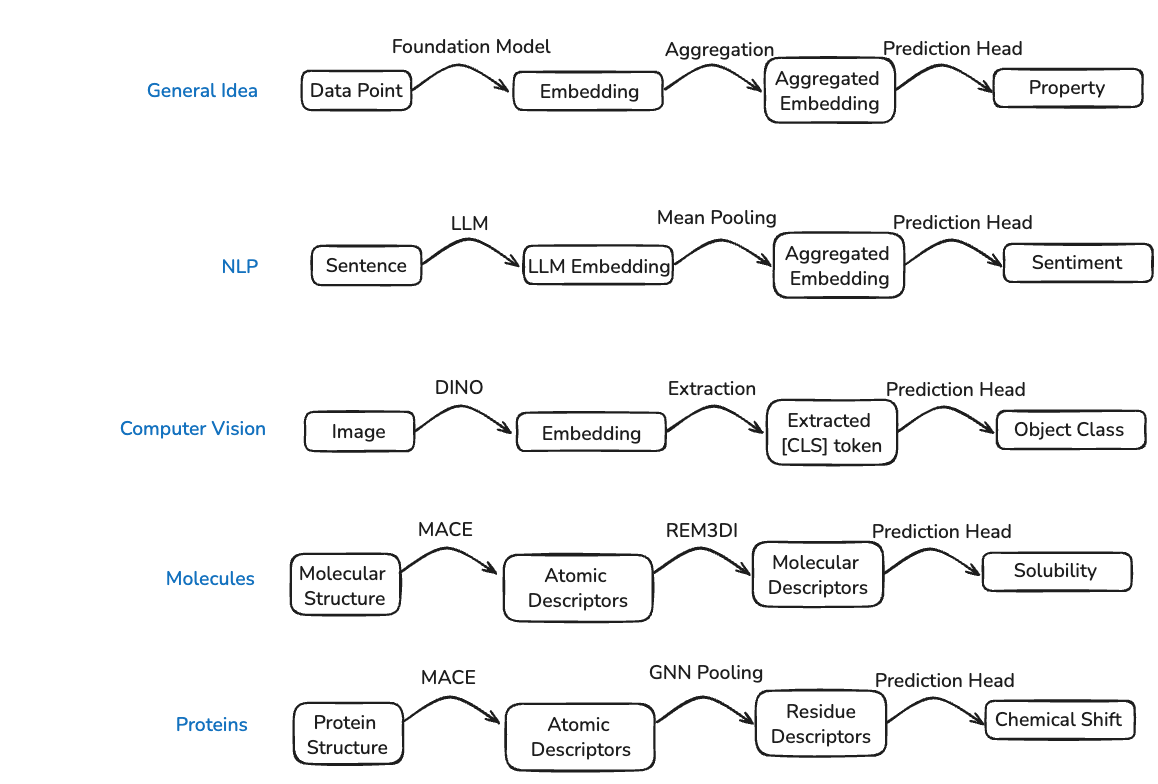Fig 17. The embedding paradigm across domains: foundation models (LLMs, DINO, MACE) produce local embeddings that are aggregated and fed to task-specific prediction heads. In molecules, MACE atomic descriptors are pooled via learned aggregators like REM3DI; in proteins, they can be pooled to residue-level descriptors via GNN pooling.

This pattern has been successfully instantiated for both molecules and proteins. REM3DI ⁸⁶ learns to aggregate MACE atomic descriptors into smooth, rotation-invariant molecular representations that achieve state-of-the-art performance on property prediction benchmarks. For proteins, similar approaches pool MACE atomic descriptors to the residue level, enabling prediction of per-residue properties like NMR chemical shifts or pKa values⁸⁷.

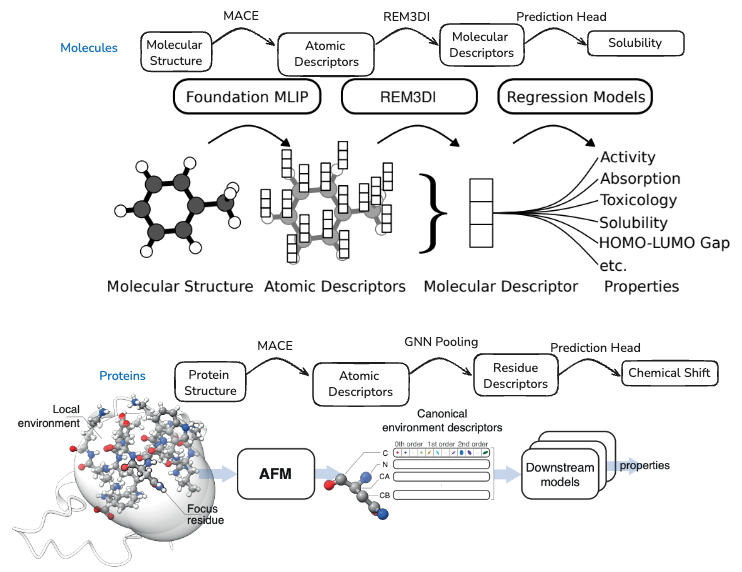
Fig 18. Left: REM3DI aggregates MACE atomic descriptors into molecular descriptors for property prediction. Right: MACE atomic descriptors can be pooled to residue-level representations for protein property prediction, extracting canonical environment descriptors from local atomic neighborhoods.

Where to Go from Here? Permalink

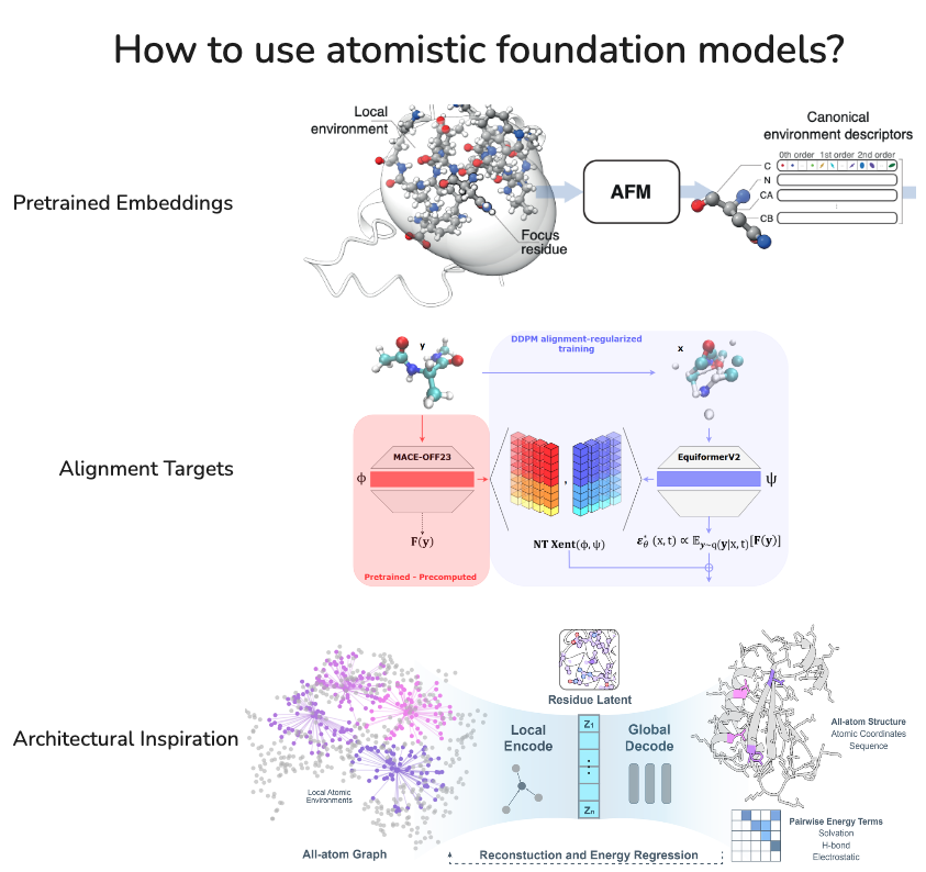Fig 19. Three complementary approaches to leveraging atomistic foundation models: (1) using pretrained embeddings directly for downstream tasks, (2) aligning generative model representations to foundation model features, and (3) drawing architectural inspiration from what makes foundation models generalise well.

Using pretrained embeddings remains powerful for property prediction, though naively incorporating them does not seem to help structure prediction—as we explored in the RF3 paper ⁹¹, simply conditioning on MACE embeddings did not improve structure prediction accuracy. Representation alignment (as in MACE-REPA) has started but remains in its infancy compared to the sophisticated alignment methods developed for images.

A third, perhaps underexplored angle is architectural inspiration: why does MACE work so well and generalise so broadly? Three factors likely contribute: (1) training on large-scale DFT data, (2) physics-grounded objectives (energies and forces), and (3) strong locality bias—MACE operates on strictly local atomic environments rather than global molecular graphs. SLAE ⁹² takes exactly this approach for proteins: it adopts the physics-grounded objective by predicting Rosetta energy terms (hydrogen bonding, solvation, electrostatics) and embraces strict locality by encoding all-atom environments rather than full protein graphs. This places SLAE conceptually close to aligned VAEs in vision—reconstruction ensures geometric fidelity while auxiliary physics heads encourage the latent space to align with physically meaningful axes.

Conclusion Permalink

The field has undergone rapid evolution, progressing through four distinct phases: (1) aligning diffusion features with pretrained representations, (2) incorporating semantic structure into VAE latent spaces, (3) directly using pretrained representations as latent spaces, and (4) questioning whether pretrained representations are necessary at all. Parallel developments in pixel-space diffusion and generative representation learning have further enriched the landscape.

Several clear patterns emerge: representation alignment dramatically accelerates training, spatial structure may be more important than global semantics, VAE compression is not fundamental, and principles transfer beyond vision to molecular modeling. However, fundamental questions remain: What makes representations learnable? What is the optimal compression rate? How do we unify multiple modalities? Should we train jointly or in stages?

The answers likely depend on scale, application requirements, and computational constraints. At research scale, leveraging pretrained models provides clear advantages for rapid iteration and exploration. At production scale, state-of-the-art systems like FLUX, Veo, and Sora demonstrate that multi-stage latent approaches—not necessarily end-to-end training—can achieve maximum quality. This suggests that the modularity of staged training, where VAEs are pretrained and reused, offers both efficiency and quality benefits at scale. While pixel-space methods continue to advance and may avoid certain reconstruction artifacts, latent-space methods currently dominate production deployments due to their computational efficiency, which is critical when serving millions of users or generating expensive video content.

Looking forward, I am very excited to see how these advances in vision will translate to the molecular world. I myself have worked quite a bit on generative modelling for proteins ⁹³ and small molecules ⁹⁴, recently also leveraging latent diffusion ⁹⁵, so I will follow this space with great interest!

Credits Permalink

Thanks to everyone who gave feedback to this blogpost, especially Arash Vahdat, Karsten Kreis and the rest of the GenAIR team as well as members of the Baker lab for interesting discussions about this topic. Also thanks to Philip Isola and the rest of the “Foundation of Computer Vision” team for making their great text openly accessible from which I got the title image for this blogpost as well as the representation vs generation figure.

References Permalink

1. Ho, J., et al. (2020). Denoising Diffusion Probabilistic Models. NeurIPS. https://arxiv.org/abs/2006.11239 ↩︎ ↩︎²

2. Song, Y., et al. (2020). Score-Based Generative Modeling through Stochastic Differential Equations. ICLR. https://arxiv.org/abs/2011.13456 ↩︎ ↩︎²

3. Lai, C.-H., Song, Y., Kim, D., Mitsufuji, Y., & Ermon, S. (2025). The principles of diffusion models. arXiv preprint arXiv:2510.21890. https://arxiv.org/abs/2510.21890 ↩︎

4. Lipman, Y., et al. (2024). Flow Matching for Generative Modeling. ICLR. https://arxiv.org/abs/2210.02747 ↩︎ ↩︎²

5. Albergo, M. S., & Vanden-Eijnden, E. (2023). Building Normalizing Flows with Stochastic Interpolants. ICLR. https://arxiv.org/abs/2209.15571 ↩︎

6. Radford, A., et al. (2021). Learning Transferable Visual Models From Natural Language Supervision. ICML. https://arxiv.org/abs/2103.00020 ↩︎ ↩︎² ↩︎³

7. Caron, M., et al. (2021). Emerging Properties in Self-Supervised Vision Transformers. ICCV. https://arxiv.org/abs/2104.14294 ↩︎ ↩︎² ↩︎³

8. He, K., et al. (2022). Masked Autoencoders Are Scalable Vision Learners. CVPR. https://arxiv.org/abs/2111.06377 ↩︎ ↩︎² ↩︎³

9. Kadkhodaie, Z., Mallat, S., & Simoncelli, E. (2025). Unconditional CNN denoisers contain sparse semantic representation of images. arXiv preprint arXiv:2506.01912. https://arxiv.org/abs/2506.01912 ↩︎

10. Liang, Q., Liu, Z., Ostrow, M., & Fiete, I. (2024). How Diffusion Models Learn to Factorize and Compose. arXiv preprint arXiv:2408.13256. https://arxiv.org/abs/2408.13256 ↩︎

11. Jaini, P., Clark, K., & Geirhos, R. (2024). Intriguing properties of generative classifiers. arXiv preprint arXiv:2309.16779. https://arxiv.org/abs/2309.16779 ↩︎

12. Sohl-Dickstein, J., Weiss, E., Maheswaranathan, N., & Ganguli, S. (2015). Deep unsupervised learning using nonequilibrium thermodynamics. International Conference on Machine Learning, 2256–2265. https://arxiv.org/abs/1503.03585 ↩︎

13. Song, Y., & Ermon, S. (2020). Improved techniques for training score-based generative models. Advances in neural information processing systems, 33, 12438–12448. ↩︎

14. Vahdat, A., & Kautz, J. (2020). NVAE: A Deep Hierarchical Variational Autoencoder. NeurIPS. https://arxiv.org/abs/2007.03898 ↩︎

15. Vahdat, A., et al. (2021). Score-based generative modeling in latent space. NeurIPS. https://arxiv.org/abs/2106.05931 ↩︎ ↩︎²

16. Rombach, R., et al. (2022). High-Resolution Image Synthesis with Latent Diffusion Models. CVPR. https://arxiv.org/abs/2112.10752 ↩︎ ↩︎²

17. Dieleman, S. (2025). Generative modelling in latent space. https://sander.ai/2025/04/15/latents.html ↩︎ ↩︎²

18. Blattmann, A., et al. (2023). Align your Latents: High-Resolution Video Synthesis with Latent Diffusion Models. CVPR. https://arxiv.org/abs/2304.08818 ↩︎

19. Brooks, T., et al. (2024). Video generation models as world simulators. OpenAI Blog. https://openai.com/index/video-generation-models-as-world-simulators/ ↩︎ ↩︎² ↩︎³

20. Podell, D., et al. (2023). SDXL: Improving Latent Diffusion Models for High-Resolution Image Synthesis. ICLR. https://arxiv.org/abs/2307.01952 ↩︎

21. Peebles, W., & Xie, S. (2023). Scalable Diffusion Models with Transformers. ICCV. https://arxiv.org/abs/2212.09748 ↩︎

22. Gao, R., Hoogeboom, E., Heek, J., Bortoli, V. D., Murphy, K. P., & Salimans, T. (2024). Diffusion meets flow matching: Two sides of the same coin. arXiv preprint arXiv:2401.08740. https://arxiv.org/abs/2401.08740 ↩︎

23. Esser, P., et al. (2024). Scaling Rectified Flow Transformers for High-Resolution Image Synthesis. ICML. https://arxiv.org/abs/2403.03206 ↩︎ ↩︎²

24. Oord, A. v. d., Li, Y., & Vinyals, O. (2019). Representation Learning with Contrastive Predictive Coding. arXiv preprint arXiv:1807.03748. https://arxiv.org/abs/1807.03748 ↩︎ ↩︎² ↩︎³

25. Chen, X., & He, K. (2020). Exploring Simple Siamese Representation Learning. CVPR. https://arxiv.org/abs/2011.10566 ↩︎ ↩︎²

26. Caron, M., et al. (2019). Deep Clustering for Unsupervised Learning of Visual Features. ECCV. https://arxiv.org/abs/1807.05520 ↩︎ ↩︎²

27. Caron, M., et al. (2021). Unsupervised Learning of Visual Features by Contrasting Cluster Assignments. NeurIPS. https://arxiv.org/abs/2006.09882 ↩︎ ↩︎²

28. Assran, M., et al. (2023). Self-Supervised Learning from Images with a Joint-Embedding Predictive Architecture. CVPR. https://arxiv.org/abs/2301.08243 ↩︎ ↩︎² ↩︎³

29. Huh, M., Cheung, B., Wang, T., & Isola, P. (2024). The Platonic Representation Hypothesis. arXiv preprint arXiv:2405.07987. https://arxiv.org/abs/2405.07987 ↩︎ ↩︎² ↩︎³ ↩︎⁴ ↩︎⁵

30. Chen, T., et al. (2020). A Simple Framework for Contrastive Learning of Visual Representations. ICML. https://arxiv.org/abs/2002.05709 ↩︎ ↩︎²

31. Oquab, M., et al. (2024). DINOv2: Learning Robust Visual Features without Supervision. arXiv preprint arXiv:2304.07193. https://arxiv.org/abs/2304.07193 ↩︎ ↩︎² ↩︎³

32. Simeoni, O., et al. (2025). DINOv3. arXiv preprint arXiv:2508.10104. https://arxiv.org/abs/2508.10104 ↩︎ ↩︎²

33. Assran, M., et al. (2025). V-JEPA 2: Self-Supervised Video Models Enable Understanding, Prediction and Planning. arXiv preprint arXiv:2506.09985. https://arxiv.org/abs/2506.09985 ↩︎

34. Zhai, X., et al. (2023). Sigmoid Loss for Language Image Pre-Training. ICCV. https://arxiv.org/abs/2303.15343 ↩︎ ↩︎²

35. Tschannen, M., et al. (2025). SigLIP 2: Multilingual Vision-Language Encoders with Improved Semantic Understanding, Localization, and Dense Features. arXiv preprint arXiv:2502.14786. https://arxiv.org/abs/2502.14786 ↩︎

36. Grill, J.-B., et al. (2020). Bootstrap Your Own Latent: A New Approach to Self-Supervised Learning. NeurIPS. https://arxiv.org/abs/2006.07733 ↩︎

37. Richemond, P. H., et al. (2020). BYOL works even without batch statistics. arXiv preprint arXiv:2010.10241. https://arxiv.org/abs/2010.10241 ↩︎

38. Skorokhodov, I., et al. (2025). Improving the Diffusability of Autoencoders. arXiv preprint arXiv:2502.14831. https://arxiv.org/abs/2502.14831 ↩︎ ↩︎² ↩︎³

39. Chen, H., et al. (2025). Masked Autoencoders Are Effective Tokenizers for Diffusion Models. arXiv preprint arXiv:2502.03444. https://arxiv.org/abs/2502.03444 ↩︎ ↩︎² ↩︎³

40. Zhou, J., et al. (2021). iBOT: Image BERT Pre-Training with Online Tokenizer. ICLR. https://arxiv.org/abs/2111.07832 ↩︎

41. Gupta, S., Sundaram, S., Wang, C., Jegelka, S., & Isola, P. (2025). Better Together: Leveraging Unpaired Multimodal Data for Stronger Unimodal Models. arXiv preprint arXiv:2510.08492. https://arxiv.org/abs/2510.08492 ↩︎

42. Wang, S. L., Isola, P., & Cheung, B. (2025). Words That Make Language Models Perceive. arXiv preprint arXiv:2510.02425. https://arxiv.org/abs/2510.02425 ↩︎ ↩︎²

43. Bi, T., Zhang, X., Lu, Y., & Zheng, N. (2025). Vision Foundation Models Can Be Good Tokenizers for Latent Diffusion Models. arXiv preprint arXiv:2510.18457. https://arxiv.org/abs/2510.18457 ↩︎ ↩︎²

44. Yu, S., et al. (2025). Representation Alignment for Generation: Training Diffusion Transformers Is Easier Than You Think. arXiv preprint arXiv:2410.06940. https://arxiv.org/abs/2410.06940 ↩︎ ↩︎² ↩︎³

45. Wu, G., et al. (2025). Representation Entanglement for Generation: Training Diffusion Transformers Is Much Easier Than You Think. arXiv preprint arXiv:2507.01467. https://arxiv.org/abs/2507.01467 ↩︎ ↩︎²

46. Leng, X., Singh, J., Hou, Y., Xing, Z., Xie, S., & Zheng, L. (2025). REPA-E: Unlocking VAE for End-to-End Tuning with Latent Diffusion Transformers. arXiv preprint arXiv:2504.10483. https://arxiv.org/abs/2504.10483 ↩︎ ↩︎²

47. Yao, J., Yang, B., & Wang, X. (2025). Reconstruction vs. Generation: Taming Optimization Dilemma in Latent Diffusion Models. arXiv preprint arXiv:2501.01423. https://arxiv.org/abs/2501.01423 ↩︎ ↩︎²

48. Wang, Z., et al. (2025). REPA Works Until It Doesn’t: Early-Stopped, Holistic Alignment Supercharges Diffusion Training. arXiv preprint arXiv:2505.16792. https://arxiv.org/abs/2505.16792 ↩︎ ↩︎²

49. Wang, R., & He, K. (2025). Diffuse and Disperse: Image Generation with Representation Regularization. arXiv preprint arXiv:2506.09027. https://arxiv.org/abs/2506.09027 ↩︎ ↩︎²

50. Xiang, W., et al. (2023). Denoising Diffusion Autoencoders are Unified Self-Supervised Learners. ICCV. https://arxiv.org/abs/2303.09769 ↩︎

51. Chen, X., Liu, Z., Xie, S., & He, K. (2024). Deconstructing denoising diffusion models for self-supervised learning. arXiv preprint arXiv:2401.14404. https://arxiv.org/abs/2401.14404 ↩︎

52. Singh, J., Leng, X., Wu, Z., Zheng, L., Zhang, R., Shechtman, E., & Xie, S. (2025). What matters for Representation Alignment: Global Information or Spatial Structure? arXiv preprint arXiv:2512.10794. https://arxiv.org/abs/2512.10794 ↩︎ ↩︎²

53. Shechtman, E., & Irani, M. (2007). Matching local self-similarities across images and videos. 2007 IEEE Conference on Computer Vision and Pattern Recognition (pp. 1–8). IEEE. https://ieeexplore.ieee.org/document/4270170 ↩︎

54. Dieleman, S. (2023). The geometry of diffusion guidance. https://sander.ai/2023/08/28/geometry.html ↩︎

55. Goodfellow, I., et al. (2014). Generative Adversarial Networks. NeurIPS. https://arxiv.org/abs/1406.2661 ↩︎

56. Chen, B., et al. (2025). Aligning Visual Foundation Encoders to Tokenizers for Diffusion Models. arXiv preprint arXiv:2509.25162. https://arxiv.org/abs/2509.25162 ↩︎

57. Bolya, D., et al. (2025). Perception Encoder: The best visual embeddings are not at the output of the network. arXiv preprint arXiv:2504.13181. https://arxiv.org/abs/2504.13181 ↩︎

58. Shi, M., et al. (2025). Latent Diffusion Model without Variational Autoencoder. arXiv preprint arXiv:2510.15301. https://arxiv.org/abs/2510.15301 ↩︎

59. Zheng, B., Ma, N., Tong, S., & Xie, S. (2025). Diffusion Transformers with Representation Autoencoders. arXiv preprint arXiv:2510.11690. https://arxiv.org/abs/2510.11690 ↩︎

60. Zhai, S., Zhang, R., Nakkiran, P., Berthelot, D., Gu, J., Zheng, H., Chen, T., Bautista, M. A., Jaitly, N., & Susskind, J. (2024). Normalizing flows are capable generative models. arXiv preprint arXiv:2412.06329. https://arxiv.org/abs/2412.06329 ↩︎

61. Gao, Y., Chen, C., Chen, T., & Gu, J. (2025). One Layer Is Enough: Adapting Pretrained Visual Encoders for Image Generation. arXiv preprint arXiv:2512.07829. https://arxiv.org/abs/2512.07829 ↩︎

62. Tong, S., Zheng, B., Wang, Z., Tang, B., Ma, N., Brown, E., Yang, J., Fergus, R., LeCun, Y., & Xie, S. (2026). Scaling Text-to-Image Diffusion Transformers with Representation Autoencoders. arXiv preprint arXiv:2601.16208. https://arxiv.org/abs/2601.16208 ↩︎

63. Kumar, A., & Patel, V. M. (2026). Learning on the Manifold: Unlocking Standard Diffusion Transformers with Representation Encoders. arXiv preprint arXiv:2602.10099. https://arxiv.org/abs/2602.10099 ↩︎

64. Mathieu, E., & Nickel, M. (2020). Riemannian Continuous Normalizing Flows. Advances in Neural Information Processing Systems, 33, 2503-2515. https://arxiv.org/abs/2006.10605 ↩︎

65. Zaghen, O., Eijkelboom, F., Pouplin, A., & Bekkers, E. J. (2025). Towards Variational Flow Matching on General Geometries. arXiv preprint arXiv:2502.12981. https://arxiv.org/abs/2502.12981 ↩︎

66. Bamberger, J., Jones, I., Duncan, D., Bronstein, M. M., Vandergheynst, P., & Gosztolai, A. (2025). Carré du champ flow matching: better quality-generalisation tradeoff in generative models. arXiv preprint arXiv:2510.05930. https://arxiv.org/abs/2510.05930 ↩︎

67. Zhang, S. (2025). Both Semantics and Reconstruction Matter: Making Representation Encoders Ready for Text-to-Image Generation and Editing. arXiv preprint arXiv:2509.25162. https://arxiv.org/abs/2509.25162 ↩︎

68. Fan, W., Diao, H., Wang, Q., Lin, D., & Liu, Z. (2025). The Prism Hypothesis: Harmonizing Semantic and Pixel Representations via Unified Autoencoding. arXiv preprint arXiv:2512.19693. https://arxiv.org/abs/2512.19693 ↩︎

69. Falck, F., et al. (2025). Spectral Autoencoders. arXiv preprint arXiv:2505.11278. https://arxiv.org/abs/2505.11278 ↩︎

70. Chu, X., Li, R., & Wang, Y. (2025). USP: Unified Self-Supervised Pretraining for Image Generation and Understanding. arXiv preprint arXiv:2503.06132. https://arxiv.org/abs/2503.06132 ↩︎

71. Black Forest Labs. (n.d.). FLUX. https://bfl.ai/research/representation-comparison ↩︎

72. Li, T., & He, K. (2025). Back to Basics: Let Denoising Generative Models Denoise. arXiv preprint arXiv:2511.13720. https://arxiv.org/abs/2511.13720 ↩︎

73. Yu, Y., Xiong, W., Nie, W., Sheng, Y., Liu, S., & Luo, J. (2025). PixelDiT: Pixel Diffusion Transformers for Image Generation. arXiv preprint arXiv:2511.20645. https://arxiv.org/abs/2511.20645 ↩︎

74. Ma, Z., Wei, L., Wang, S., Zhang, S., & Tian, Q. (2025). DeCo: Frequency-Decoupled Pixel Diffusion for End-to-End Image Generation. arXiv preprint arXiv:2511.19365. https://arxiv.org/abs/2511.19365 ↩︎

75. Chen, Z., et al. (2025). DiP: Taming Diffusion Models in Pixel Space. arXiv preprint arXiv:2511.18822. https://arxiv.org/abs/2511.18822 ↩︎

76. Hoogeboom, E., Mensink, T., Heek, J., Lamerigts, K., Gao, R., & Salimans, T. (2025). Simpler Diffusion (SiD2): 1.5 FID on ImageNet512 with pixel-space diffusion. arXiv preprint arXiv:2410.19324. https://arxiv.org/abs/2410.19324 ↩︎

77. Lei, J., Liu, K., Berner, J., Yu, H., Zheng, H., Wu, J., & Chu, X. (2025). Advancing End-to-End Pixel Space Generative Modeling via Self-supervised Pre-training. arXiv preprint arXiv:2510.12586. https://arxiv.org/abs/2510.12586 ↩︎ ↩︎²

78. El-Nouby, A., Klein, M., Zhai, S., Bautista, M. A., Toshev, A., Shankar, V., Susskind, J. M., & Joulin, A. (2024). Scalable pre-training of large autoregressive image models. arXiv preprint arXiv:2401.08541. https://arxiv.org/abs/2401.08541 ↩︎

79. Chen, M., et al. (2020). Generative Pretraining from Pixels. ICML. https://arxiv.org/abs/2009.14794 ↩︎

80. Ren, S., Wang, Z., Zhu, H., Xiao, J., Yuille, A., & Xie, C. (2023). Rejuvenating image-gpt as strong visual representation learners. arXiv preprint arXiv:2312.02147. https://arxiv.org/abs/2312.02147 ↩︎

81. Fini, E., Shukor, M., Li, X., Dufter, P., Klein, M., Haldimann, D., Aitharaju, S., da Costa, V. G. T., Béthune, L., Gan, Z., et al. (2025). Multimodal autoregressive pre-training of large vision encoders. Proceedings of the Computer Vision and Pattern Recognition Conference, 9641-9654. https://arxiv.org/abs/2502.14786 ↩︎

82. Xu, S., Ma, Z., Chai, W., Chen, X., Jin, W., Chai, J., Xie, S., & Yu, S. X. (2025). Next-Embedding Prediction Makes Strong Vision Learners. arXiv preprint arXiv:2512.16922. https://arxiv.org/abs/2512.16922 ↩︎

83. Lei, J., Berner, J., Wang, J., Chen, Z., Ba, Z., Ren, K., Zhu, J., & Anandkumar, A. (2025). Robust Representation Consistency Model via Contrastive Denoising. arXiv preprint arXiv:2501.13094. https://arxiv.org/abs/2501.13094 ↩︎

84. Batatia, I., et al. (2025). A foundation model for atomistic materials chemistry. The Journal of Chemical Physics, 163(18). https://arxiv.org/abs/2406.11627 ↩︎

85. Bernstein, N. (2024). From GAP to ACE to MACE. arXiv preprint arXiv:2410.06354. https://arxiv.org/abs/2410.06354 ↩︎

86. Wedig, S., Elijošius, R., Schran, C., & Schaaf, L. L. (2025). REM3DI: Learning smooth, chiral 3D molecular representations from equivariant atomistic foundation models. NeurIPS 2025 Workshop on Symmetry and Geometry in Neural Representations. https://arxiv.org/abs/2506.11627 ↩︎ ↩︎²

87. Bojan, M., Vedula, S., Maddipatla, A., Sellam, N. B., Napoli, F., Schanda, P., & Bronstein, A. M. (2025). Representing local protein environments with atomistic foundation models. arXiv preprint arXiv:2505.23354. https://arxiv.org/abs/2505.23354 ↩︎ ↩︎²

88. Edamadaka, S., Yang, S., Li, J., & Gómez-Bombarelli, R. (2025). Universally Converging Representations of Matter Across Scientific Foundation Models. arXiv preprint arXiv:2512.03750. https://arxiv.org/abs/2512.03750 ↩︎

89. Li, Z., & Walsh, A. (2025). Platonic representation of foundation machine learning interatomic potentials. arXiv preprint arXiv:2512.05349. https://arxiv.org/abs/2512.05349 ↩︎

90. Pinede, L., Yang, S., Nam, J., & Gomez-Bombarelli, R. (2025). Unifying Force Prediction and Molecular Conformation Generation Through Representation Alignment. ICML 2025 Generative AI and Biology (GenBio) Workshop. https://openreview.net/pdf?id=yzkHGHvC74 ↩︎

91. Corley, N., Mathis, S., Krishna, R., Bauer, M. S., Thompson, T. R., Ahern, W., …, Didi, K., …, Baker, D., & DiMaio, F. (2025). Accelerating Biomolecular Modeling with AtomWorks and RF3. bioRxiv. https://www.biorxiv.org/content/10.1101/2025.08.14.670328v2 ↩︎

92. Chen, Y., Lu, T., Zhao, C., Wayment-Steele, H., & Huang, P. (2025). SLAE: Strictly Local All-atom Environment for Protein Representation. bioRxiv. https://www.biorxiv.org/content/10.1101/2025.10.03.680398v1 ↩︎

93. Geffner, T., Didi, K., Zhang, Z., Reidenbach, D., Cao, Z., Yim, J., Geiger, M., Dallago, C., Kucukbenli, E., Vahdat, A., & others. (2025). Proteina: Scaling flow-based protein structure generative models. arXiv preprint arXiv:2503.00710. https://arxiv.org/abs/2503.00710 ↩︎

94. Schneuing, A., Harris, C., Du, Y., Didi, K., Jamasb, A., Igashov, I., Du, W., Gomes, C., Blundell, T. L., Lio, P., & others. (2024). Structure-based drug design with equivariant diffusion models. Nature Computational Science, 4(12), 899–909. https://www.nature.com/articles/s43588-024-00737-x ↩︎

95. Geffner, T., Didi, K., Cao, Z., Reidenbach, D., Zhang, Z., Dallago, C., Kucukbenli, E., Kreis, K., & Vahdat, A. (2025). La-proteina: Atomistic protein generation via partially latent flow matching. arXiv preprint arXiv:2507.09466. https://arxiv.org/abs/2507.09466 ↩︎